4  Sampling

PDF version

4.1 Data

Consider a dataset \{X_1, \ldots, X_n\} with n observations or individuals i = 1, \ldots, n. Each observation X_i consists of k variables or measurements, i.e., X_i is a k \times 1 vector X_i = (X_{i1}, X_{i2}, \ldots , X_{ik})' \in \mathbb R^k.

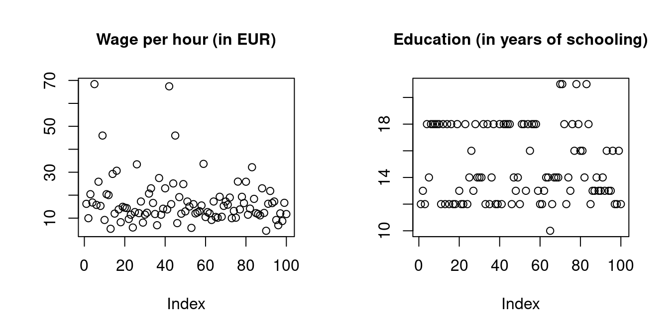
For instance, let’s consider a sub-sample of n=100 observations of the 2021 German General Social Survey (ALLBUS) of the variables wage and education.

Click here to see the dataset

Table 4.1: ALLBUS data sub-sample

Person	Wage	Education
1	16.23	12
2	9.96	13
3	20.43	12
4	16.80	18
5	68.39	14
6	15.76	18
7	25.86	18
8	15.33	18
9	45.98	18
10	9.20	18
11	20.43	12
12	20.04	18
13	5.35	12
14	29.26	18
15	11.97	12
16	30.65	18
17	13.79	12
18	8.21	12
19	14.94	18
20	14.55	13
21	14.37	12
22	9.62	12
23	11.49	18
24	5.91	12
25	12.64	14
26	33.44	16
27	12.17	13
28	17.24	18
29	8.05	14
30	11.54	14
31	12.36	14
32	20.69	18
33	22.99	12
34	16.61	18
35	11.79	12
36	6.90	14
37	27.47	18
38	11.49	12
39	14.10	12
40	22.99	18
41	13.79	12
42	67.43	18
43	16.09	18
44	25.11	18
45	45.98	18
46	7.82	12
47	19.16	14
48	11.93	13
49	24.83	14
50	12.93	12
51	17.24	18
52	15.05	18
53	5.75	13
54	16.09	18
55	12.04	16
56	12.48	18
57	13.05	18
58	15.52	18
59	33.64	13
60	10.48	12
61	12.64	12
62	12.07	13
63	9.20	14
64	17.24	14
65	10.51	10
66	10.16	12
67	19.31	14
68	10.61	14
69	15.33	14
70	17.24	21
71	15.87	21
72	18.97	18
73	9.96	12
74	13.14	14
75	10.18	13
76	25.91	18
77	13.79	16
78	19.29	21
79	16.55	18
80	25.86	16
81	11.49	16
82	14.15	14
83	32.18	21
84	18.39	18
85	12.18	12
86	11.78	13
87	11.20	13
88	22.99	14
89	12.26	13
90	4.48	13
91	16.26	14
92	21.84	13
93	16.55	16
94	17.24	13
95	9.20	13
96	6.90	16
97	12.07	12
98	8.73	12
99	16.67	16
100	11.77	12

We have a dataset of n=100 bivariate observation vectors X_i = \begin{pmatrix} W_i \\ S_i \end{pmatrix}, \quad i=1, \ldots, 100, where W_i and S_i are the wage level and years of schooling of individual i.

From the perspective of empirical analysis, a dataset is simply an array of numbers that are fixed and presented to a researcher.

From the perspective of statistical theory, a dataset consists of n repeated realizations of a k-variate random variable X with distribution F. In the above case, we have X = (W, S)', where W and S are random variables for wage and education.

The distribution F is called population distribution. The population can be thought of as an infinitely large group of hypothetical individuals from which we draw our data rather than a fixed group of a physical population. A finite physical population would be the 83 million inhabitants of Germany. An infinite population is a theoretical auxiliary construct. For example, one can imagine the infinite group of potentially born persons with all their possible characteristics.

A parameter is a feature (function) of the population distribution F, such as expectations, variances, or correlations. Statistical analysis is concerned with inference on parameters of the population distribution F.

4.2 Random sampling

In statistical analysis, a dataset \{X_1, \ldots, X_n\} that is drawn from some population F is also called sample.

The ALLBUS data are cross-sectional data, where n individuals are randomly selected from the German population and independently interviewed on k variables. The ALLBUS data consists of n independently replicated random experiments.

i.i.d. sample / random sample

A collection of random vectors \{X_1, \ldots, X_n\} is i.i.d. (independent and identically distributed) if X_i and X_j are mutually independent and have the same distribution F for all i \neq j.

An i.i.d. dataset or i.i.d. sample is also called a random sample. F is called population distribution or data-generating process (DGP).

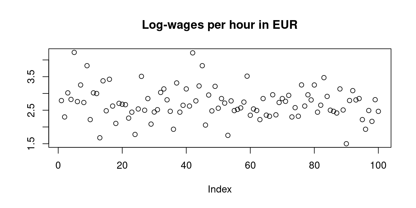
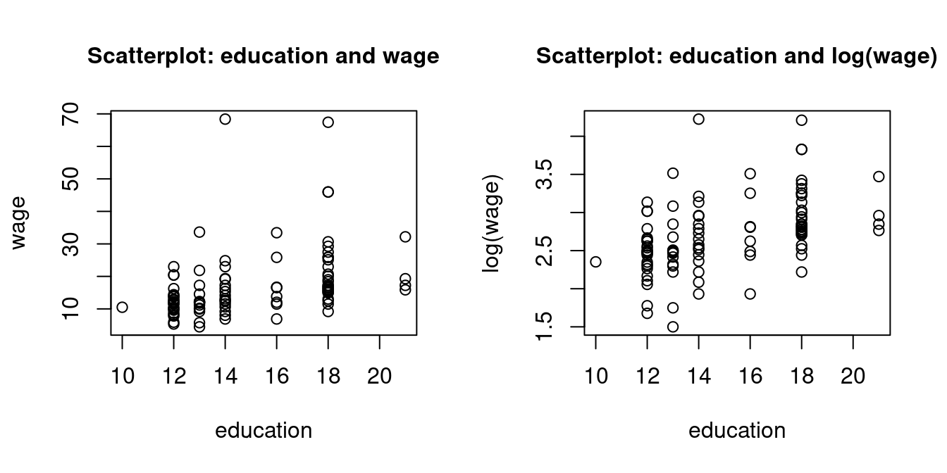
Any transformed sample \{g(X_1), \ldots, g(X_n)\} of an i.i.d. sample \{X_1, \ldots, X_n\} is also an i.i.d. sample (g may be any function). For instance, we may consider the log-transformed data, which produces a less skewed and fat-tailed distribution:

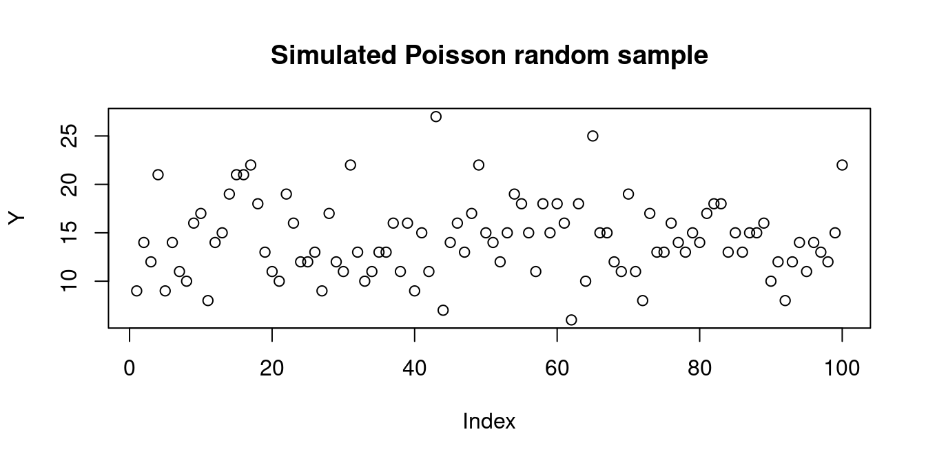
Below, you find a simulated random sample from a Poisson distribution with parameter \lambda = 14:

Y = rpois(100, 14)
plot(Y, main="Simulated Poisson random sample")

Statistical analysis is concerned with inference on parameters of the population distribution F from which the data is sampled.

Sampling methods of obtaining economic datasets that may be considered as random sampling are:

• Survey sampling
  Examples: representative survey of randomly selected households from a list of residential addresses; online questionnaire to a random sample of recent customers
• Administrative records
  Examples: data from a government agency database, Statistisches Bundesamt, ECB, etc.
• Direct observation
  Collected data without experimental control and interactions with the subject. Example: monitoring customer behavior in a retail store
• Web scraping
  Examples: collected house prices on real estate sites or hotel/electronics prices on booking.com/amazon, etc.
• Field experiment
  To study the impact of a treatment or intervention on a treatment group compared with a control group. Example: testing the effectiveness of a new teaching method by implementing it in a selected group of schools and comparing results to other schools with traditional methods
• Laboratory experiment
  Example: a controlled medical trial for a new drug

4.3 Dependent sampling

Examples of cross-sectional data sampling that may produce some dependence across observations are:

• Stratified sampling
  The population is first divided into homogenous subpopulations (strata), and a random sample is obtained from each stratum independently. Examples: divide companies into industry strata (manufacturing, technology, agriculture, etc.) and sample from each stratum; divide the population into income strata (low-income, middle-income, high-income).
  The sample is independent within each stratum, but it is not between different strata. The strata are defined based on specific characteristics that may be correlated with the variables collected in the sample.

• Clustered sampling
  Entire subpopulations are drawn. Example: new teaching methods are compared to traditional ones on the student level, where only certain classrooms are randomly selected, and all students in the selected classes are evaluated.
  Within each cluster (classroom), the sample is dependent because of the shared environment and teacher’s performance, but between classrooms, it is independent.

Other types of data we often encounter in econometrics are time series data, panel data, or spatial data:

• Time series data consists of observations collected at different points in time, such as stock prices, daily temperature measurements, or GDP figures. These observations are ordered and typically show temporal trends, seasonality, and autocorrelation.

• Panel data involves observations collected on multiple entities (e.g., individuals, firms, countries) over multiple time periods.

• Spatial data includes observations taken at different geographic locations, where values at nearby locations are often correlated.

Time series, panel, and spatial data cannot be considered a random sample given their temporal or geographic dependence.

4.4 Time series data

Time series data \{Y_1, \ldots, Y_n\} is a sequence of real-valued observations arranged chronologically and indexed by time. In contrast to cross-sectional data, we typically use the index t to indicate the observation index, i.e., we write Y_t for the time t observation.

The order defined by the time indices is essential to time series data. We usually expect observations close in time to be strongly dependent and observations at greater distances to be less dependent. It is a fundamental difference to cross-sectional data, where each index represents an individual, and the ordering of the indices is interchangeable.

The time series process is the underlying doubly infinite sequence of random variables \{ Y_t \}_{t \in \mathbb Z} = \{ \ldots, Y_{-1}, Y_0, \underbrace{Y_1, \ldots, Y_n}_{\text{observed part}}, Y_{n+1}, \ldots \}. where the time series sample \{Y_1, \ldots, Y_n\} is only the observed part of the process.

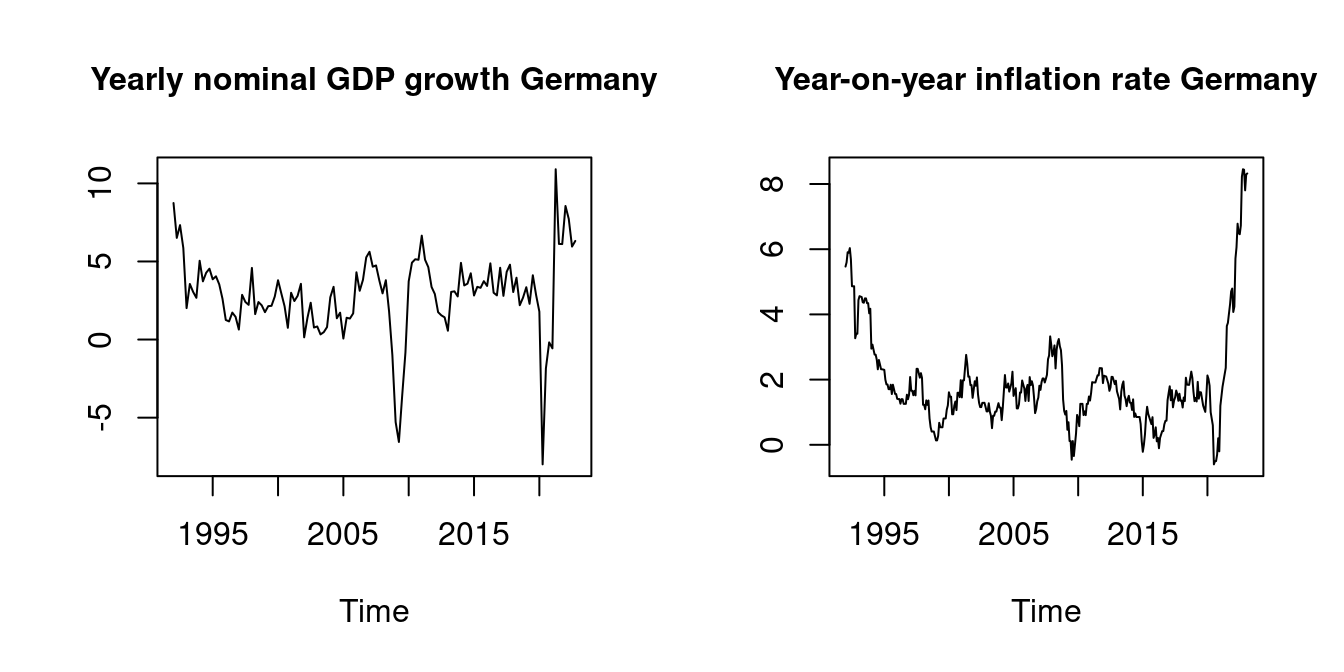
Examples of time series data are the nominal GDP growth and the inflation rate of Germany.

Stationary time series

A time series Y_t is called stationary if the mean \mu and the autocovariances \gamma(\tau) do not depend on the time point t. That is, \mu := E[Y_t] < \infty, \quad \text{for all} \ t, and \gamma(\tau) := Cov(Y_t, Y_{t-\tau}) < \infty \quad \text{for all} \ t \ \text{and} \ \tau.

The function \gamma(\cdot) of a stationary time series Y_t is called autocovariance function, and \gamma(\tau) is the autocovariance of order \tau. The autocorrelation of order \tau is \rho(\tau) = \frac{Cov(Y_t, Y_{t-\tau})}{Var[Y_t]}, \quad \tau \in \mathbb Z.

The autocorrelations of stationary time series typically decay to zero quite quickly as \tau increases. If \rho(\tau) \to 0 as \tau \to \infty quickly enough so that \sum_{\tau=1}^\infty \rho(\tau) < \infty, the time series is called a short memory time series. For short memory time series, observations close in time may be highly correlated, but observations farther apart have little dependence.

One of the most commonly studied time series processes is the autoregressive process of order one with parameter \phi. It is defined as Y_t = c + \phi Y_{t-1} + u_t, where \{u_t\} is an i.i.d. process of increments with E[u_t] = 0 and Var[u_t] = \sigma_u^2, and c is a constant. If |\phi| < 1, the AR(1) process is stationary with \mu = \frac{c}{1-\phi}, \quad \gamma(\tau) = \frac{\phi^\tau \sigma_u^2}{1-\phi^2}, \quad \rho(\tau) = \phi^\tau, \quad \tau \geq 0. Its autocorrelations \rho(\tau) = \phi^\tau decay exponentially in the lag order \tau.

u = rnorm(250)
AR1 = stats::filter(u, 0.8, "recursive")
plot(AR1, main=expression(paste("Simulated AR(1) process with ",varphi,"=0.8 and standard normal increments")), ylab = "")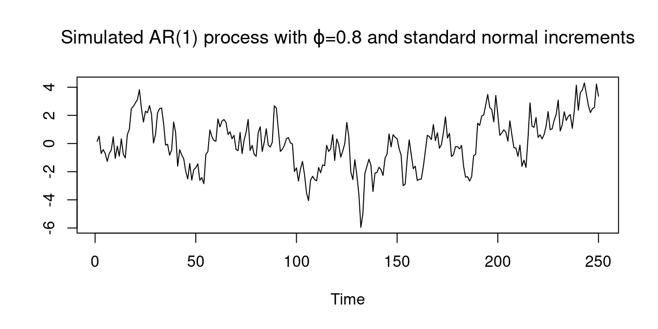

More complex time dependencies can be modeled using an AR(p) process Y_t = c + \phi_1 Y_{t-1} + \ldots + \phi_p Y_{t-p} + u_t. Many macroeconomic time series, such as GDP growth or inflation rates can be modeled using autoregressive processes.

A time series Y_t is nonstationary if the mean E[Y_t] or the autocovariances Cov(Y_t, Y_{t-\tau}) change with t, i.e., if there exist time points s \neq t with E[Y_t] \neq E[Y_s] \quad \text{or} \quad Cov(Y_t,Y_{t-\tau}) \neq Cov(Y_s,Y_{s-\tau}) for some \tau.

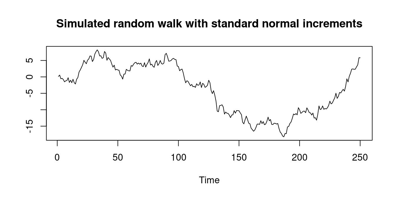
The simple random walk is an example of a nonstationary time series process. It is an AR(1) process with \phi=1, c=0, and starting value Y_0 = 0, i.e., Y_t = Y_{t-1} + u_t, \quad t \geq 1. By backward substitution, it can be expressed as the cumulative sum Y_t = \sum_{j=1}^t u_j.

It is nonstationary since Cov(Y_t, Y_{t-\tau}) = (t-\tau) \sigma_u^2, which depends on t and becomes larger as t gets larger.

RW = stats::filter(u, 1, "recursive")
plot(RW, main= "Simulated random walk with standard normal increments", ylab = "")

4.5 Additional reading

• Stock and Watson (2019), Sections 1-2, 15
• Hansen (2022a), Section 6
• Hansen (2022b), Section 3
• Davidson and MacKinnon (2004), Section 1

4.6 R-codes

statistics-sec4.R