Call:
lm(formula = wage ~ female, data = allbus21)

Coefficients:
(Intercept)       female
17.618 -3.139 plot(fitted.values(fit1), residuals(fit1))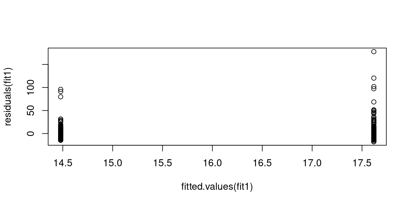
The previous section discussed OLS regression from a descriptive perspective. A regression model puts the regression problem into a stochastic framework.
Linear Regression Model
Let \{(Y_i, X_i'), i=1, \ldots, n \} be a sample from some joint population distribution, where Y_i is individual i’s dependent variable, and X_i = (1, X_{i2}, \ldots, X_{ik})' is the k \times 1 vector of individual i’s regressor variables.
The linear regression model equation for i=1, \ldots, n is Y_i = \beta_1 + \beta_2 X_{i2} + \ldots + \beta_k X_{ik} + u_i \tag{10.1} where \beta = (\beta_1, \ldots, \beta_k)' is the k \times 1 vector of regression coefficients and u_i is the error term for individual i.
In vector notation, we write Y_i = X_i'\beta + u_i, \quad i=1, \ldots, n.
The error term represents further factors that affect the dependent variable and are not included in the model. These factors include measurement errors, omitted variables, or unobserved/unmeasurable variables.
We can use matrix notation to describe the n individual regression equations jointly: The regressor matrix and the response vector are \underset{(n\times 1)}{\boldsymbol Y} = \begin{pmatrix} Y_1 \\ Y_2 \\ \vdots \\ Y_n \end{pmatrix}, \quad \underset{(n\times k)}{\boldsymbol X} = \begin{pmatrix} X_1' \\ X_2' \\ \vdots \\ X_n' \end{pmatrix} = \begin{pmatrix} 1 & X_{12} & \ldots & X_{1k} \\ \vdots & & & \vdots \\ 1 & X_{n2} &\ldots & X_{nk} \end{pmatrix} The vectors of coefficients and error terms are \underset{(k\times 1)}{\beta} = \begin{pmatrix} \beta_1 \\ \vdots \\ \beta_k \end{pmatrix}, \quad \underset{(n\times 1)}{\boldsymbol u} = \begin{pmatrix} u_1 \\ \vdots \\ u_n \end{pmatrix}. In matrix notation, the i=1, \ldots, n equations from Equation 10.1 can be jointly written as \boldsymbol Y = \boldsymbol X \beta + \boldsymbol u.
A1: Mean independence condition
E[u_i \mid X_i] = 0 \tag{10.2}
Equation 10.2 is also called conditional mean assumption or weak exogeneity condition. It is the condition that essentially makes Equation 10.1 a regression model. It has multiple implications.
Equation 10.2 and the LIE imply E[u_i] \overset{\tiny (LIE)}{=} E[\underbrace{E[u_i \mid X_i]}_{=0}] = E[0] = 0 The error term has a zero unconditional mean: E[u_i] = 0.
The conditional mean of Y_i given X_{i} is E[Y_i \mid X_i] = \underbrace{E[X_i'\beta \mid X_i]}_{\overset{\tiny (CT)}{=} X_i'\beta} + \underbrace{E[u_i \mid X_i]}_{=0} = X_i'\beta.
A regression model is a model for the conditional expectation of the response given the regressors. A linear regression model assumes that the conditional expectation is linear.
Recall the best predictor property of the conditional expectation. The regression function X_i'\beta is the best predictor for Y_i given X_i (assuming that E[Y_i^2] < \infty).
E[Y_i \mid X_i] = X_i'\beta = \beta_1 + \beta_2 X_{i2} + \ldots + \beta_k X_{ik} implies \frac{\text{d} E[Y_i \mid X_i]}{ \text{d} X_{ij}} = \beta_j The coefficient \beta_j is the marginal effect holding all other regressors fixed (partial derivative).
Note that the marginal effect \beta_j is not necessarily a causal effect of X_{ij} on Y_i. Unobserved variables that are correlated with X_{ij} might be the actual “cause” of the change in Y_i.
For any regressor variable X_{ij}, j=1, \ldots, k, we have E[u_i \mid X_{ij}] \overset{\tiny (LIE)}{=} E[\underbrace{E[u_i \mid X_i]}_{=0} \mid X_{ij}] = 0 and E[X_{ij} u_i] \overset{\tiny (LIE)}{=} E[E[X_{ij} u_i \mid X_{ij}]] \overset{\tiny (CT)}{=} E[X_{ij} \underbrace{E[u_i \mid X_{ij}]}_{=0}] = 0, which implies Cov(X_{ij},u_i) = \underbrace{E[X_{ij} u_i]}_{=0} - E[X_{ij}] \underbrace{E[u_i]}_{=0} = 0. The error term is uncorrelated with all regressor variables. The regressors are called exogenous. Therefore, the condition E[u_i \mid X_i] = 0 is also called weak exogeneity condition.
It implies that the error term describes only the unobserved variables that are uncorrelated with the regressors. Note that it does not mean that we exclude any effects on the dependent variable of unobserved variables that are correlated with the regressors (which is a quite likely situation).
The exogeneity condition only tells us that the marginal effect \beta_j is an average effect of a change in X_{ij}, holding all other regressors fixed. We cannot hold fixed the unobserved variables that are correlated with X_{ij}. Any effects of unobserved variables that are correlated with the j-th regressor are implicitly part of the model since they enter the marginal effect \beta_j through their correlation with X_{ij}.
Let’s consider, for example, the wage per hour on education regression model:
wage_i = \beta_1 + \beta_2 \ edu_i + u_i, \quad E[u_i \mid edu_i] = 0, \quad i=1, \ldots, n. We have E[wage_i \mid edu_i] = \beta_1 + \beta_2 edu_i. The average wage level among all individuals with z years of schooling is \beta_1 + \beta_2 z. The marginal effect of education is \frac{\text{d} E[wage_i \mid edu_i]}{\text{d} \ edu_i} = \beta_2.
Interpretation: Suppose that \beta_2 = 1.5. People with one more year of education are paid on average 1.50 EUR more than people with one year less of education.
Cov(wage_i, edu_i) = Cov(\beta_1 + \beta_2 edu_i, edu_i) + \underbrace{Cov(u_i, edu_i)}_{=0} = \beta_2 Var[edu_i] The coefficient \beta_2 is \beta_2 = \frac{Cov(wage_i, edu_i)}{Var[edu_i]} = Corr(wage_i, edu_i) \cdot \frac{sd(wage_i)}{sd(edu_i)} It describes the correlative relationship between education and wages. It makes no statement about where exactly a higher wage level for people with more education comes from. Regression coefficients do not necessarily yield causal conclusions.
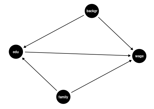
Maybe people with more education are just smarter on average and therefore earn more on average. Or maybe people with more education have richer parents on average and, therefore, have jobs with higher salaries. Or maybe education really does help to increase wages.
The coefficient \beta_2 is high when the correlation between education and wage is high.
This could be due to family background (parental education, family income, ethnicity, structural racism) if family background correlates with wage and education.
Or it could be due to personal background (gender, intelligence) if personal background correlates with wage and education.
Of course, it could also be due to an actual high causal effect of education on wages.
Perhaps it is a mixture of different effects. We cannot disentangle these effects unless we include additional control variables.
Notice: Correlation does not imply causation!
Suppose the research question is to understand the causal effect of an additional year of education on wages, with family and personal background held fixed. In that case, family and personal background are so-called omitted variables.
A variable is an omitted variable if
If omitted variables are present, we say that we have an omitted variable bias for the causal effect of the regressor of interest. Omitted variables imply that we cannot interpret the coefficient \beta_2 as a causal effect. It is simply a correlative effect or marginal effect. This must always be kept in mind when interpreting regression coefficients This
We can include control variables in the linear regression model to reduce the omitted variables so that we can interpret \beta_2 as a ceteris paribus marginal effect (ceteris paribus means with other variables held constant). For instance, we can include the experience in years and the ethnicity and gender dummy variables for Black and female: wage_i = \beta_1 + \beta_2 edu_i +\beta_3 exp_i + \beta_4 Black_i + \beta_5 female_i + u_i In this case, \beta_2 = \frac{\text{d} E[wage_i \mid edu_i, exp_i, Black_i, female_i]}{\text{d} \ edu_i} is the marginal effect of education on expected wages, holding constant experience, ethnicity, and gender.
But: it does not hold constant further unobservable characteristics (such as ability) nor variables not included in the regression (such as quality of education), so an omitted variaable bias might still be present.
A linear relationship is not always appropriate. E.g., it is not reasonable that an individual with one year of education has the same marginal effect of education on average wages as an individual with 20 years of education. It would make more sense if the marginal effect were a percentage change.
In the level specification wage_i = \beta_1 + \beta_2 edu_i + u_i the parameter \beta_2 approximates an absolute change in wage when education changes by 1: \frac{\text{d} \ wage_i}{\text{d} \ edu_i} = \beta_2 \quad \Rightarrow \quad \underbrace{\text{d} \ wage_i}_{\approx \text{absolute change}} = \beta_2 \underbrace{\text{d} \ edu_i}_{\approx \text{absolute change}}
In the logarithmic specification \log(wage_i) = \beta_1 + \beta_2 edu_i + u_i the parameter \beta_2 approximates the percentage change in wage when education changes by 1: \begin{align*} wage_i &= e^{\beta_1 + \beta_2 edu_i + u_i} \\ \Rightarrow \qquad \frac{\text{d} \ wage_i}{\text{d} \ edu_i} &= \beta_2 e^{\beta_1 + \beta_2 edu_i + u_i} = \beta_2 \ wage_i \\ \Rightarrow \qquad \underbrace{\frac{\text{d} \ wage_i}{wage_i}}_{\approx \ \substack{\text{percentage} \\ \text{change}}} &= \beta_2 \underbrace{\text{d} \ edu_i}_{\approx \ \text{absolute change} } \end{align*}
For instance, if \beta_2 = 0.05, then a person with one more year of education has, on average, a 5% higher wage.
The linear regression model is less restrictive than it appears. It can represent nonlinearities very flexibly since we can include as regressors nonlinear transformations of the original regressors.
A linear regression with quadratic and interaction terms \begin{align*} wage_i = \beta_1 &+ \beta_2 edu_i + \beta_3 exp_i + \beta_4 exp^2_i \\ &+ \beta_5 female_i + \beta_6 married_i + \beta_7 (married_i \cdot female_i) + u_i \end{align*}
Marginal effects depend on the person’s experience level/marital status/gender: \begin{align*} \frac{\text{d} \ wage_i}{\text{d} \ exp_i} &= \beta_3 + 2 \beta_4 exp_i \\ \frac{\text{d} \ wage_i}{\text{d} \ female_i} &= \beta_5 + \beta_7 married_i \\ \frac{\text{d} \ wage_i}{\text{d} \ married_i} &= \beta_6 + \beta_7 female_i \end{align*}
Reall that the exogeneity condition E[u_i \mid X_i]=0 implies E[X_{ij} u_i]=0 for all j=1,\dots,k. Thus, the exogeneity condition gives us a system of k linear equations: \left. \begin{array}{c} E[u_i]=0\\ E[X_{i2} u_i]=0\\ \vdots\\ E[X_{ik} u_i]=0 \end{array} \right\}\quad \Leftrightarrow \quad \underset{(k\times 1)}{E[X_i u_i]}=\underset{(k\times 1)}{\boldsymbol 0_k}
It allows us to identify the unknown parameter vector \beta\in\mathbb{R}^k in terms of population moments: \begin{align*} E[X_i(\underbrace{Y_i - X_i'\beta}_{=u_i})] &= \boldsymbol 0_k \\ E[X_i Y_i] - E[X_i X_i']\beta &= \boldsymbol 0_k \\ E[X_iX_i']\beta &= E[X_iY_i] \\ \beta &= (E[X_iX_i'])^{-1} E[X_i Y_i] \end{align*}
The regression coefficent vector \beta is a function of E[X_iX_i'] and E[X_iY_i], which are population moments of the (k+1)-variate random variable (Y_i, X_i'). The corresponding sample moments are \frac{1}{n} \sum_{i=1}^n X_iX_i' and \frac{1}{n} \sum_{i=1}^n X_i Y_i. The moment estimator for \beta substitutes population moments by sample moments: \hat\beta_{mm} = \bigg(\frac{1}{n}\sum_{i=1}^n X_iX_i'\bigg)^{-1} \frac{1}{n}\sum_{i=1}^n X_iY_i, It can be simplified as follows: \begin{align*} \hat\beta_{mm} & = \bigg(\frac{1}{n}\sum_{i=1}^n X_iX_i'\bigg)^{-1} \frac{1}{n}\sum_{i=1}^n X_iY_i \\ & = \bigg(\sum_{i=1}^n X_iX_i'\bigg)^{-1} \sum_{i=1}^n X_iY_i\\ & = \big(\boldsymbol X' \boldsymbol X\big)^{-1} \boldsymbol X' \boldsymbol Y = \widehat \beta. \end{align*}
Thus, the method of moments estimator, \hat\beta_{mm}, coincides with the OLS coefficient vector \widehat \beta. Therefore, we call \widehat \beta = \hat\beta_{mm} the OLS estimator for \beta.
A2: Random sampling
The (k+1)-variate observations \{(Y_i, X_i'), i=1, \ldots, n \} are an i.i.d. sample from some joint population distribution.
The i.i.d. assumption (A2) implies that \{(Y_i,X_i',u_i), i=1,\ldots,n\} is an i.i.d. collection since u_i = Y_i - X_i'\beta is a function of a random sample, and functions of independent variables are independent as well. Individual i’s error term u_i is independent of u_j, X_j, and Y_j for any other individual j \neq i.
This implies that the weak exogeneity condition (A1) turns into a strict exogeneity property: E[u_i \mid \boldsymbol X] = E[u_i \mid X_1, \ldots, X_n] \overset{\tiny (A2)}{=} E[u_i \mid X_i] \overset{\tiny (A1)}{=} 0. \tag{10.3} Weak exogeneity means that individual i’s regressors are uncorrelated with individual i’s error term. Strict exogeneity means that individual i’s regressors are uncorrelated with the error terms of any individual in the sample.
Strict exogeneity is a property in a regression model with randomly sampled data, but it may not hold in dynamic time series regression models with an autocorrelated response variable.
A dynamic time series model is a model where one of the regressors is a lag of the dependent variable. For instance, the model Y_t = \beta_1 + \beta_2 X_t + u_t, \quad E[u_t \mid X_t] = 0, with X_t = Y_{t-1} is called AR(1) dynamic regression model. Since Cov(Y_t, u_t) = \beta_2 \underbrace{Cov(X_t, u_t)}_{=0} + Cov(u_t, u_t) = Var[u_t] \neq 0 and X_{t+1} = Y_t, we have Cov(u_t, X_{t+1}) \neq 0. Hence, weak exogeneity (Equation 10.2) holds in dynamic time series models, but strict exogeneity (Equation 10.3) does not.
For regressions with time series data, the following alternative assumption is made:
A2b: Weak dependence
The (k+1)-variate observations \{(Y_t, X_t'), t=1, \ldots, n \} are a stationary short-memory time series, and (Y_t, X_t') and (Y_{t-\tau}, X_{t-\tau}') become independent as \tau gets large.
The precise mathematical statement for A2b is omitted. It essentially requires that the dependent variable and the regressors together have a time-independent autocovariance structure (no structural changes, no non-stationarities) and that the dependence on the time series of \tau periods before must decrease with higher \tau.
The i.i.d. assumption (A2) is not as restrictive as it may seem at first sight. It allows for dependence between u_i and X_i = (X_{i1},\dots,X_{ik})'. The error term u_i can have a conditional distribution that depends on X_i.
The exogeneity assumption (A1) requires that the conditional mean of u_i is independent of X_i. Besides this, dependencies between u_i and X_{i1},\dots,X_{ik} are allowed. For instance, the variance of u_i can be a function of X_{i1},\dots,X_{ik}. If this is the case, u_i is said to be heteroskedastic.
Let’s have a look at the conditional covariance matrix \boldsymbol D := Var[\boldsymbol u \mid \boldsymbol X] = E[\boldsymbol u \boldsymbol u' \mid \boldsymbol X].
(A2) implies E[u_i \mid u_j, \boldsymbol X] = E[u_i \mid \boldsymbol X] = 0 for j \neq i and, therefore, E[u_i u_j \mid \boldsymbol X] \overset{\tiny (LIE)}{=} E\big[E[u_i u_j \mid u_j, \boldsymbol X] \mid \boldsymbol X\big] \overset{\tiny (CT)}{=} E\big[u_j \underbrace{E[u_i \mid u_j, \boldsymbol X]}_{=0} \mid \boldsymbol X\big] = 0. Hence, u_i and u_j are conditionally uncorrelated. The off-diagonal elements of \boldsymbol D are zero.
The main diagonal elements of \boldsymbol D are E[u_i^2 \mid \boldsymbol X] \overset{\tiny (A2)}{=} E[u_i^2 \mid X_i] =: \sigma_i^2 = \sigma^2(X_i). The conditional variances of u_i may depend on the values of X_i. We have \boldsymbol D = E[\boldsymbol u \boldsymbol u' \mid \boldsymbol X] = \begin{pmatrix} \sigma_1^2 & 0 & \ldots & 0 \\ 0 & \sigma_2^2 & \ldots & 0 \\ \vdots & \vdots & \ddots & \vdots \\ 0 & 0 & \ldots & \sigma_n^2 \end{pmatrix} = diag(\sigma_1^2, \ldots, \sigma_n^2).
Homoskedastic and heteroskedastic errors
An error term is heteroskedastic if the conditional variances Var[u_i \mid X_i = x_i] = \sigma^2(X_i) are equal to a non-constant variance function \sigma^2(x_i) > 0, which is a function of the value of the regressor X_i = x_i.
An error term is homoskedastic if the conditional variances Var[u_i \mid X_i = x_i] = \sigma^2 = Var[u_i] are equal to some constant \sigma^2 > 0 for every possible regressor realization X_i = x_i.
Homoskedastic errors are a restrictive assumption sometimes made for convenience in addition to (A1)+(A2). Homoskedasticity is often unrealistic in practice, so we stick with the heteroskedastic errors framework.
Example (wages and gender):
It may be the case that there is more variation in the wage levels of male workers than in the wage levels of female workers. I.e., \{(wage_i, female_i), \ i=1, \ldots, n\} may be an i.i.d. sample that follows the regression model wage_i = \beta_1 + \beta_2 female_i + u_i, \quad E[u_i \mid female_i] = 0, where Var[u_i \mid female_i] = (1 - 0.4 female_i) \sigma^2 = \sigma^2_i, and female_i is a dummy variable. Male workers have an error variance of \sigma^2, and female workers have an error variance of 0.6 \sigma^2. The conditional error variance depends on the regressor value, i.e., the errors are heteroskedastic.
If the proportion of female and male workers is 50/50 (i.e. P(female_i = 1) = 0.5), the unconditional variance is \begin{align*} Var[u_i] &= E[u_i^2] \\ &= E[E[u_i^2 \mid female_i]] \\ &= \sigma^2 \cdot 0.5 + 0.6 \sigma^2 \cdot 0.5 \\ &= 0.8 \sigma^2. \end{align*}
Let’s have a look at what the data tells us. We use data from the Allbus21 survey.
Call:
lm(formula = wage ~ female, data = allbus21)
Coefficients:
(Intercept) female
17.618 -3.139 plot(fitted.values(fit1), residuals(fit1))The plot shows the residuals \widehat{u}_i plotted against the fitted values \widehat{Y}_i. The residuals for male workers have more variation than those for female workers, which indicates heteroskedasticity.
Another example - regressing food expenditure on income:
# install.packages("remotes")
# remotes::install_github("ccolonescu/PoEdata")
library(PoEdata) # for the "food" dataset contained in this package
data("food")     # makes the dataset "food" usable

fit2 = lm(food_exp ~ income, data = food)
## Diagnostic scatter plot of residuals vs fitted values
plot(fitted.values(fit2), residuals(fit2))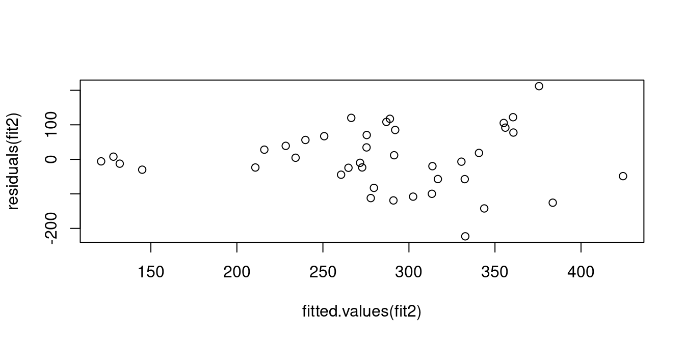
The diagnostic plot indicates that the variance of unobserved factors for food expenditure is higher for people with high income than those with low income.
Note: Plotting against the fitted values is actually a pretty smart idea since this also works for multiple predictors X_{i1},\dots,X_{ik} with k\geq 3.
For historical reasons, statistics books often treat homoskedasticity as the standard case and heteroskedasticity as a special case. However, this does not reflect empirical practice since we have to expect heteroskedastic errors in most applications. It turns out that heteroskedasticity is not a problem as long as the correct inference method is chosen (robust standard errors). We will consider heteroskedasticity as the standard case and homoskedasticity as a restrictive special case.
Recall that (A1) and (A2) imply the strict exogeneity and heteroskedasticity property: E[\boldsymbol u \mid \boldsymbol X] = \boldsymbol 0_n, \quad Var[\boldsymbol u \mid \boldsymbol X] = \boldsymbol D = diag(\sigma_1^2, \ldots, \sigma_n^2). To compute the bias and MSE of the OLS estimator \widehat \beta for \beta, the following decomposition is useful: \begin{align*} \widehat \beta &= (\boldsymbol X' \boldsymbol X)^{-1} \boldsymbol X' \boldsymbol Y \\ &= (\boldsymbol X' \boldsymbol X)^{-1} \boldsymbol X' (\boldsymbol X \beta + \boldsymbol u) \\ &= (\boldsymbol X' \boldsymbol X)^{-1} (\boldsymbol X' \boldsymbol X) \beta + (\boldsymbol X' \boldsymbol X)^{-1} \boldsymbol X' \boldsymbol u \\ &= \beta + (\boldsymbol X' \boldsymbol X)^{-1} \boldsymbol X' \boldsymbol u \end{align*}
The linear regression model is a conditional model, so let’s first compute the mean and variance of \widehat \beta conditional on all regressors of all individuals \boldsymbol X.
\begin{align*} E[\widehat \beta \mid \boldsymbol X] & = \beta + E[(\boldsymbol X' \boldsymbol X)^{-1} \boldsymbol X' \boldsymbol u \mid \boldsymbol X] \\ & \overset{\tiny (CT)}{=} (\boldsymbol X' \boldsymbol X)^{-1} \boldsymbol X' \underbrace{E[\boldsymbol u \mid \boldsymbol X]}_{= \boldsymbol 0} = \beta \end{align*}
The OLS estimator is unbiased conditional on \boldsymbol X, which means that the estimator is unbiased for any realization of the regressors. Unbiased conditional on \boldsymbol X is a stronger concept than unconditional unbiasedness since, by the LIE, E[\widehat \beta] = E[ \underbrace{E[\widehat \beta \mid \boldsymbol X]}_{= \beta} ] = \beta. Hence, the OLS estimator is unbiased: bias[\widehat \beta] = 0.
Recall the matrix rule Var[\boldsymbol A \boldsymbol z] = \boldsymbol A Var[\boldsymbol z] \boldsymbol A' if \boldsymbol z is a random vector and \boldsymbol A is a matrix. Then, the conditional sampling variance is \begin{align*} Var[\widehat \beta \mid \boldsymbol X] &= Var[\beta + (\boldsymbol X'\boldsymbol X)^{-1} \boldsymbol X' \boldsymbol u \mid \boldsymbol X] \\ &= Var[(\boldsymbol X'\boldsymbol X)^{-1} \boldsymbol X' \boldsymbol u \mid \boldsymbol X] \\ &= (\boldsymbol X'\boldsymbol X)^{-1} \boldsymbol X' Var[\boldsymbol u \mid \boldsymbol X] ((\boldsymbol X'\boldsymbol X)^{-1} \boldsymbol X')' \\ &= (\boldsymbol X'\boldsymbol X)^{-1} \boldsymbol X' \boldsymbol D \boldsymbol X (\boldsymbol X'\boldsymbol X)^{-1} \\ &= \bigg(\sum_{i=1}^n X_i X_i'\bigg)^{-1} \bigg( \sum_{i=1}^n \sigma^2_i X_i X_i' \bigg) \bigg(\sum_{i=1}^n X_i X_i'\bigg)^{-1}. \end{align*}
It turns out that Var[\widehat \beta_j \mid \boldsymbol X] \overset{p}{\rightarrow} 0 for any j and any realization of the regressors \boldsymbol X, and \lim_{n \to \infty} Var[\widehat \beta_j] = 0.
Proof. Under the additional condition that 0 < E[X_{ij}^4] < \infty and 0 < E[Y_i^4] < \infty, it can be shown that \frac{1}{n}\sum_{i=1}^n X_i X_i' \overset{p}{\rightarrow} E[X_iX_i'] =: \boldsymbol Q and \frac{1}{n}\sum_{i=1}^n \sigma^2_i X_i X_i' \overset{p}{\rightarrow} E[(X_iu_i)(X_i u_i)'] =: \boldsymbol \Omega, where the matrices \boldsymbol Q and \boldsymbol \Omega are positive definite if there is no strict multicollinearity. Then, \begin{align*} Var[\widehat \beta \mid \boldsymbol X] &= \bigg(\sum_{i=1}^n X_i X_i'\bigg)^{-1} \bigg( \sum_{i=1}^n \sigma^2_i X_i X_i' \bigg) \bigg(\sum_{i=1}^n X_i X_i'\bigg)^{-1} \\ &= \underbrace{\frac{1}{n}}_{\to 0} \bigg(\underbrace{\frac{1}{n}\sum_{i=1}^n X_i X_i'}_{\overset{p}{\rightarrow} \boldsymbol Q}\bigg)^{-1} \bigg(\underbrace{\frac{1}{n} \sum_{i=1}^n \sigma^2_i X_i X_i'}_{\overset{p}{\rightarrow} \boldsymbol \Omega} \bigg) \bigg(\underbrace{\frac{1}{n}\sum_{i=1}^n X_i X_i'}_{\overset{p}{\rightarrow} \boldsymbol Q}\bigg)^{-1}, \end{align*} which implies that Var[\widehat \beta \mid \boldsymbol X] \overset{p}{\rightarrow} \boldsymbol 0_{k \times k}, as n \to \infty. Some mathematical tools are required to show the steps rigorously (Cauchy-Schwarz inequality, Slutsky’s theorem, continuous mapping theorem).
Since \widehat \beta_j is unbiased and the conditional variance converges to zero, the unconditional variance also converges to zero. \square
Since, for any j=1, \ldots, k, bias[\widehat \beta_j] = 0 and Var[\widehat \beta_j] \to 0 as n \to \infty, we have \lim_{n \to \infty} MSE[\widehat \beta_j] = 0, which implies that the OLS estimator is consistent.
In the above steps, we required that the fourth moments of the population distribution of (Y_i, X_i') are bounded, or equivalently, that the kurtosis of the population from which the data is sampled is finite. That is, fat-tailed population distributions are not permitted.
A3: Large outliers are unlikely
Response and regressor variables have nonzero finite fourth moments: 0 < E[Y_i^4] < \infty, \quad 0 < E[X_{ij}^4] < \infty for all j = 1, \ldots, k.
Another condition that we implicitly used is that the OLS estimator can be computed. I.e., strict multicollinearity is not allowed:
A4: No perfect multicollinearity
The regressor matrix \boldsymbol X has full column rank.
The linear regression model Equation 10.1 under assumptions (A1)–(A4) is called heteroskedastic linear regression model.
OLS consistency
Under assumptions (A1)–(A4), the OLS estimator \widehat \beta is consistent for \beta. It is unbiased, and its conditional variance is \begin{align*} Var[\widehat \beta \mid \boldsymbol X] &= (\boldsymbol X'\boldsymbol X)^{-1} \boldsymbol X' \boldsymbol D \boldsymbol X (\boldsymbol X'\boldsymbol X)^{-1} \\ &= \bigg(\sum_{i=1}^n X_i X_i'\bigg)^{-1} \bigg( \sum_{i=1}^n \sigma_i^2 X_i X_i' \bigg) \bigg( \sum_{i=1}^n X_i X_i' \bigg)^{-1}. \end{align*}
It turns out that the OLS estimator is not the most efficient estimator unless the errors are homoskedastic.
A5: Homoskedasticity
The conditional variance of the errors does not depend on the realized regressors: Var[u_i \mid X_i] = \sigma^2, \quad \text{for all} \ i=1, \ldots, n.
The linear regression model Equation 10.1 under assumptions (A1)–(A5) is called homoskedastic linear regression model.
An estimator \widehat \theta is more efficient that an estimator \widehat \varphi if Var[\widehat \theta] < Var[\widehat \varphi]. If \widehat \theta and \widehat \varphi are vectors, their variances are matrices, and the expression Var[\widehat \theta] < Var[\widehat \varphi] means that (Var[\widehat \varphi] - Var[\widehat \theta]) is a positive definite matrix (see matrix tutorial)
Gauss-Markov theorem
In the homoskedastic linear regression model, the OLS estimator \widehat \beta is the best linear unbiased estimator (BLUE) for \beta. That is, for any other linear unbiased estimator \widetilde \beta, we have \begin{align*} Var[\widetilde \beta \mid X] \geq Var[\widehat \beta \mid X] \end{align*}
We call the LS estimator \hat \beta the efficient estimator in the homoskedastic linear regression model. Homoskedastic errors imply that \sigma_i^2 = \sigma^2 for all i = 1, \ldots, n so that the conditional variance simplifies in this case to
\begin{align*} Var[\widehat \beta \mid \boldsymbol X] &= \bigg(\sum_{i=1}^n X_i X_i'\bigg)^{-1} \bigg( \sum_{i=1}^n \underbrace{\sigma_i^2}_{=\sigma^2} X_i X_i' \bigg) \bigg( \sum_{i=1}^n X_i X_i' \bigg)^{-1} \\ &= \sigma^2 \bigg(\sum_{i=1}^n X_i X_i'\bigg)^{-1} \bigg( \sum_{i=1}^n X_i X_i' \bigg) \bigg( \sum_{i=1}^n X_i X_i' \bigg)^{-1} \\ &= \sigma^2 \bigg(\sum_{i=1}^n X_i X_i'\bigg)^{-1} \\ &= \sigma^2 (\boldsymbol X' \boldsymbol X)^{-1}. \end{align*}
In the heteroskedastic linear regression model, OLS is not efficient. We can recover the Gauss-Markov efficiency in the heteroskedastic linear regression model if we use the generalized least squares estimator (GLS) instead: \begin{align*} \widehat \beta_{gls} &= (\boldsymbol X' \boldsymbol D^{-1} \boldsymbol X)^{-1} \boldsymbol X' \boldsymbol D^{-1} \boldsymbol Y \\ &= \bigg( \sum_{i=1}^n \frac{1}{\sigma_i^2} X_i X_i' \bigg)^{-1} \bigg( \sum_{i=1}^n \frac{1}{\sigma_i^2} X_i Y_i \bigg), \end{align*} where \boldsymbol D = Var[\boldsymbol u \mid \boldsymbol X] = \text{diag}(\sigma_1^2, \ldots, \sigma_n^2).
The GLS estimator is BLUE in the heteroskedastic linear regression model.
However, GLS is not feasible in practice since \sigma_1^2, \ldots, \sigma_n^2 are unknown. These quantities can be estimated, but this is another source of uncertainty, and further assumptions are required (feasible GLS - FGLS). Therefore, most practitioners prefer to use the OLS estimator under heteroskedasticity and are willing to accept the loss of efficiency compared to GLS.
A6: Normal errors
The conditional distribution of u_i given X_i is \mathcal N(0, \sigma^2). That is, the conditional density of u_i given X_i = x_i is f_{u_i|X_i}(z\mid x) = \frac{1}{\sqrt{2 \pi \sigma^2}} \exp \Big( -\frac{1}{2 \sigma^2} z^2 \Big)
The condition means that the conditional distribution of the errors given the regressors is normal and does not depend on them: \begin{align*} f_{u_i|X_i}(z\mid x) = \frac{1}{\sqrt{2 \pi \sigma^2}} \exp \Big( -\frac{1}{2 \sigma^2} z^2 \Big) \end{align*}
It does not mean that the regressors are normally distributed. It only means that Y_i conditional on X_i must be normal: \begin{align*} f_{Y_i|X_i}(y \mid x) &= \frac{1}{\sqrt{2 \pi \sigma^2}} \exp \Big( -\frac{1}{2 \sigma^2} (y-x'\beta)^2 \Big) \end{align*}
The linear regression model Equation 10.1 under assumptions (A1)–(A6) is called normal linear regression model.
The OLS estimator \widehat \beta is a linear function of the regressors \boldsymbol X and the errors \boldsymbol u: \widehat \beta = (\boldsymbol X' \boldsymbol X)^{-1} \boldsymbol X' \boldsymbol Y = \beta + (\boldsymbol X' \boldsymbol X)^{-1} \boldsymbol X' \boldsymbol u Conditional on \boldsymbol X, the OLS estimator is a linear combination of the errors \boldsymbol u. If \boldsymbol u conditional on \boldsymbol X is normal, then any linear combination is also normal. Hence, the distribution of \widehat \beta conditional on \boldsymbol X is normal. Recall that E[\widehat \beta \mid \boldsymbol X] = \beta, \quad E[\widehat \beta \mid \boldsymbol X] = \sigma^2 (\boldsymbol X' \boldsymbol X)^{-1}. This leads to the following result:
Exact normality
Under assumptions (A1)–(A6), the distribution of the OLS estimator conditional on the regressors \boldsymbol X is normal for any fixed sample size n with \widehat \beta \mid \boldsymbol X \sim \mathcal N\Big(\beta, \sigma^2 (\boldsymbol X' \boldsymbol X)^{-1}\Big).
Using this result, we can derive exact inference methods (confidence intervals and t-tests)
Assumptions (A5) and (A6) are quite restrictive. Dependent variables are rarely exactly normally distributed, and error variances often depend on the values of the regressors.
(A5) and (A6) are quite useful for pedagogical purposes and to understand under what situation the exact distribution of the OLS estimator can be recovered.
Similar to the sample mean case, it turns out that the restrictive assumptions are unnecessary if we are willing to accept that we can only obtain the asymptotic distribution of the estimator. Fortunately, a central limit theorem also holds for the OLS estimator under assumptions (A1)–(A4).
Asymptotic normality of OLS for i.i.d. data
Under assumptions (A1)–(A5), the asymptotic distribution of the OLS estimator is \sqrt n (\widehat \beta - \beta) \overset{D}{\longrightarrow} \mathcal N\Big(0, \sigma^2 \boldsymbol Q^{-1}\Big), where \boldsymbol Q = E[X_i X_i'] is the second moment matrix of the regressors.
Under assumptions (A1)–(A4), the asymptotic distribution of the OLS estimator is \sqrt n (\widehat \beta - \beta) \overset{D}{\longrightarrow} \mathcal N\Big(0, \boldsymbol Q^{-1} \boldsymbol \Omega \boldsymbol Q^{-1}\Big), \tag{10.4} where \boldsymbol \Omega = E\big[(X_i u_i)(X_i u_i)'\big].
Using this result, we can derive asymptotic inference methods (confidence intervals and t-tests)
We can also use the OLS estimator if the variables are time series data. In this case, we have to assume that the time series are weakly dependent in the sense of Assumption (A2b).
The linear regression model Equation 10.1 under assumptions (A1), (A2b), (A3), and (A4) is called dynamic linear regression model.
Asymptotic normality of OLS for time series data
Under assumptions (A1), (A2b), (A3), and (A4), the asymptotic distribution of the OLS estimator is \sqrt n (\widehat \beta - \beta) \overset{D}{\longrightarrow} \mathcal N\Big(0, \boldsymbol Q^{-1} \boldsymbol \Omega^* \boldsymbol Q^{-1}\Big), where \boldsymbol \Omega^* = \boldsymbol \Omega + \sum_{\tau = 1}^\infty \Big(E\big[(X_i u_i)(X_{i-\tau} u_{i-\tau})'\big] + E\big[(X_i u_i)(X_{i-\tau} u_{i-\tau})'\big]' \Big).