fit1 = lm(logwage~education)
fit1
Call:
lm(formula = logwage ~ education)

Coefficients:
(Intercept)    education
1.10721 0.09207 Regression analysis is concerned with the approximation of a dependent variable Y_i (regressand, response variable) by a function f(X_i) of a vector of independent variables X_i (regressors, predictor variables): Y_i \approx f(X_i), \quad i=1, \ldots, n.
The least squares method selects the regression function that minimizes the squared approximation error: \min_{f} \sum_{i=1}^n (Y_i - f(X_i))^2. \tag{9.1}
In linear regression, the regression function f(\cdot) is a linear function, and the minimization problem of Equation 9.1 is called ordinary least squares (OLS) problem.
We approximate the dependent variable Y_i by a linear function of k-1 independent variables X_{i2}, \ldots, X_{ik} plus an intercept: Y_i \approx b_1 + b_2 X_{i2} + \ldots + b_k X_{ik}. The regression function can be written as an inner product: f(X_i) = b_1 + b_2 X_{i2} + \ldots + b_k X_{ik} = X_i'b, with X_i = \begin{pmatrix} 1 \\ X_{i2} \\ \vdots \\ X_{ik} \end{pmatrix}, \quad b = \begin{pmatrix} b_1 \\ b_2 \\ \vdots \\ b_k \end{pmatrix}, where X_i is the vector of k regressors and b is the vector of k regression coefficients.
For a given sample \{(Y_1, X_1'), \ldots, (Y_n, X_n')\} and a given coefficient vector b \in \mathbb R^K the sum of squared errors is S_n(b) = \sum_{i=1}^n (Y_i - f(X_i))^2 = \sum_{i=1}^n (Y_i - X_i'b)^2. The least squares coefficient vector \widehat \beta is the minimizing argument: \widehat \beta = \argmin_{b \in \mathbb R^k} \sum_{i=1}^n (Y_i - X_i'b)^2 \tag{9.2}
Least squares coefficients
If the k \times k matrix (\sum_{i=1}^n X_i X_i') is invertible, the solution to Equation 9.2 is unique with \widehat \beta = \Big( \sum_{i=1}^n X_i X_i' \Big)^{-1} \sum_{i=1}^n X_i Y_i. \tag{9.3}
Proof. Write the sum of squared errors as \begin{align*} S_n(b) = \sum_{i=1}^n (Y_i - X_i'b)^2 = \sum_{i=1}^n Y_i^2 - 2 b' \sum_{i=1}^n X_i Y_i + b' \sum_{i=1}^n X_i X_i' b. \end{align*} The first-order condition for a minimum in b=\widehat \beta is that the gradient is zero, and the second-order condition is that the Hessian matrix is positive definite (see Matrix calculus).
The first-order condition \begin{align*} \frac{\partial S_n(b)}{\partial b} = -2 \sum_{i=1}^n X_i Y_i + 2 \sum_{i=1}^n X_i X_i' b \overset{!}{=} \boldsymbol 0_k \end{align*} implies \begin{align*} \sum_{i=1}^n X_i X_i' \widehat \beta = \sum_{i=1}^n X_i Y_i \quad \Leftrightarrow \quad \widehat \beta = \Big( \sum_{i=1}^n X_i X_i' \Big)^{-1} \sum_{i=1}^n X_i Y_i. \end{align*}
The second-order condition
\begin{align*}
\frac{\partial^2}{\partial b \partial b'} S_n(b) = 2 \sum_{i=1}^n X_i X_i' \overset{!}{>} 0
\end{align*} is satisfied for any b since
c'\bigg(\sum_{i=1}^n X_i X_i'\bigg)c = \sum_{i=1}^n c'X_i X_i'c = \sum_{i=1}^n \underbrace{(c'X_i)^2}_{\geq 0} > 0
for any nonzero vector c \in \mathbb R^k (see definite matrix). The strict positivity follows from the condition that \sum_{i=1}^n X_i X_i' is invertible, i.e., it is nonsingular and does not have any zero eigenvalues (see here). \square
OLS fitted values and residuals
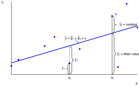
The fitted values or predicted values are \widehat Y_i = \widehat \beta_1 + \widehat \beta_2 X_{i2} + \ldots + \widehat \beta_k X_{ik} = X_i'\widehat \beta, \quad i=1, \ldots, n. The residuals are \widehat u_i = Y_i - \widehat Y_i = Y_i - X_i'\widehat \beta, \quad i=1, \ldots, n.
A simple linear regression is a linear regression of a dependent variable on a constant and a single independent variable.
Let’s revisit the wage and education data from Table 9.1 and consider only the first 20 observations:
| Person | Wage | log(Wage) | Education | Education^2 | Edu x log(wage) |
|---|---|---|---|---|---|
| 1 | 12.91 | 2.56 | 18 | 324 | 46.08 |
| 2 | 11.49 | 2.44 | 14 | 196 | 34.16 |
| 3 | 10.22 | 2.32 | 14 | 196 | 32.48 |
| 4 | 11.49 | 2.44 | 16 | 256 | 39.04 |
| 5 | 9.20 | 2.22 | 16 | 256 | 35.52 |
| 6 | 14.94 | 2.70 | 14 | 196 | 37.80 |
| 7 | 11.75 | 2.46 | 16 | 256 | 39.36 |
| 8 | 15.09 | 2.71 | 16 | 256 | 43.36 |
| 9 | 23.95 | 3.18 | 18 | 324 | 57.24 |
| 10 | 8.62 | 2.15 | 12 | 144 | 25.80 |
| 11 | 25.54 | 3.24 | 18 | 324 | 58.32 |
| 12 | 15.84 | 2.76 | 14 | 196 | 38.64 |
| 13 | 5.17 | 1.64 | 12 | 144 | 19.68 |
| 14 | 28.74 | 3.36 | 21 | 441 | 70.56 |
| 15 | 6.44 | 1.86 | 14 | 196 | 26.04 |
| 16 | 12.92 | 2.56 | 12 | 144 | 30.72 |
| 17 | 9.20 | 2.22 | 13 | 169 | 28.86 |
| 18 | 13.65 | 2.61 | 21 | 441 | 54.81 |
| 19 | 12.64 | 2.54 | 12 | 144 | 30.48 |
| 20 | 18.11 | 2.90 | 21 | 441 | 60.90 |
| sum | 277.91 | 50.87 | 312 | 5044 | 809.85 |
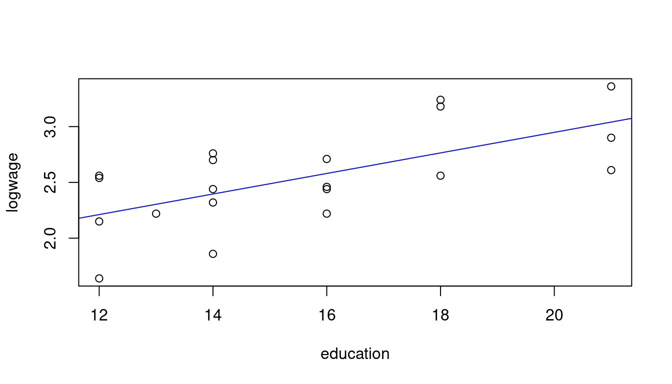
We regress Y_i = \log(wage_i) on a constant and Z_i = education_i. The regressor vector is X_i = (1,Z_i)'.
The OLS coefficients are \begin{align*} \begin{pmatrix} \hat \beta_1 \\ \hat \beta_2 \end{pmatrix} &= \Big( \sum_{i=1}^n X_i X_i' \Big)^{-1} \sum_{i=1}^n X_i Y_i \\ &= \begin{pmatrix} n & \sum_{i=1}^n Z_i \\ \sum_{i=1}^n Z_i & \sum_{i=1}^n Z_i^2 \end{pmatrix}^{-1} \begin{pmatrix} \sum_{i=1}^n Y_i \\ \sum_{i=1}^n Z_i Y_i \end{pmatrix} \end{align*}
Evaluate sums: \begin{align*} \sum_{i=1}^n X_i Y_i = \begin{pmatrix} 50.87 \\ 809.85 \end{pmatrix}, \quad \sum_{i=1}^n X_i X_i' = \begin{pmatrix} 20 & 312 \\ 312 & 5044 \end{pmatrix} \end{align*}
OLS coefficients: \begin{align*} \begin{pmatrix} \hat \beta_1 \\ \hat \beta_2 \end{pmatrix} &= \begin{pmatrix} 20 & 312 \\ 312 & 5044 \end{pmatrix}^{-1} \begin{pmatrix} 50.87 \\ 809.85 \end{pmatrix} = \begin{pmatrix} 1.107 \\ 0.092 \end{pmatrix} \end{align*}
In R, we can use the lm() function to compute the least squares coefficients:
fit1 = lm(logwage~education)
fit1
Call:
lm(formula = logwage ~ education)
Coefficients:
(Intercept) education
1.10721 0.09207 The OLS coefficient vector is \widehat \beta = (1.107, 0.092)' and the fitted regression line is f(education) = 1.107 + 0.092 \ education
par(mfrow = c(1,2))
## Fitted values and residuals
fitted = fit1$fitted.values
residuals = fit1$residuals
plot(education,fitted, main="Fitted values")
abline(fit1, col="blue")
plot(education,residuals, main="Residuals")
abline(h=0)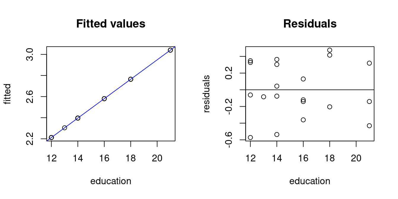
There is another, simpler formula for \widehat \beta_1 and \widehat \beta_2 in the simple linear regression model. It can be expressed in terms of sample moments:
Simple linear regression
The least squares coefficients in a simple linear regression can be written as \widehat \beta_2 = \frac{\widehat \sigma_{YZ}}{\widehat \sigma_Z^2} = \frac{s_{YZ}}{s_Z^2}, \quad \widehat \beta_1 = \overline Y - \widehat \beta_2 \overline Z \tag{9.4}
The results coincide with those from above:
beta2.hat = cov(logwage,education)/var(education)
beta1.hat = mean(logwage) - beta2.hat*mean(education)
c(beta1.hat, beta2.hat)
[1] 1.10720588 0.09207014Here is an illustration of fitted values and residuals for an OLS regression line of another dataset:
The following code computes \widehat{\beta} for a given dataset with k=3 regressors X_i = (1,X_{i2},X_{i3})':
# Some given data
Y = c(0.7,-1.0,-0.2,-1.2,-0.1,3.4,0.0,0.8,3.7,2.0)
X_2 = c(1.9,0.8,1.25,0.1,-0.1,4.4,4.6,1.6,5.5,3.4)
X_3 = c(66, 62, 59, 61, 63, 70, 68, 62, 68, 66)
## Compute the OLS estimation
fit2 = lm(Y ~ X_2 + X_3)
## Plot sample regression surface
library("scatterplot3d") # library for 3d plots
plot3d  <- scatterplot3d(x = X_2, y = X_3, z = Y,
            angle = 33, scale.y = 0.8, pch = 16,
            color ="red",
            xlab = "X_2",
            ylab = "X_3",
            main ="OLS Regression Surface")
plot3d$plane3d(fit2, lty.box = "solid", col=gray(.5), draw_polygon=TRUE)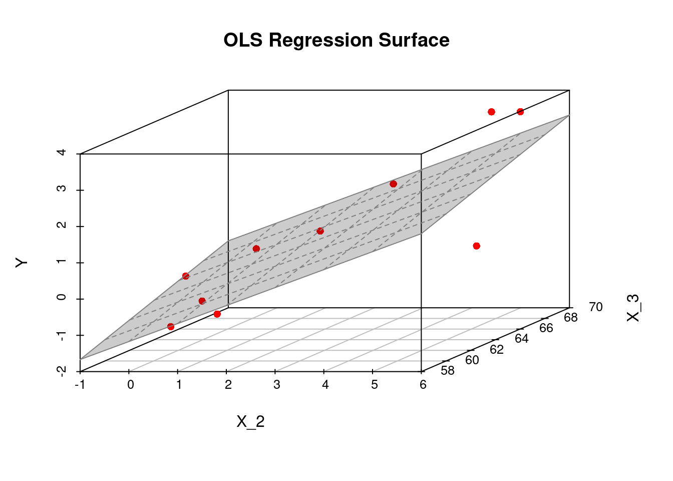
fit2$coefficients(Intercept) X_2 X_3
-8.4780709 0.4955995 0.1259828 The fitted regression surface is f(X_i) = -8.478 + 0.496 X_{i2} + 0.126 X_{i3}.
To avoid the summation notation in Equation 9.3, we stack the n observations of the dependent variable into a vector and the n regressor vectors as 1\times k row vectors into a n \times k matrix: \begin{align*} \boldsymbol Y = \begin{pmatrix} Y_1 \\ Y_2 \\ \vdots \\ Y_n \end{pmatrix}, \quad \boldsymbol X = \begin{pmatrix} X_1' \\ X_2' \\ \vdots \\ X_n' \end{pmatrix} = \begin{pmatrix} 1 & X_{12} & \ldots & X_{1k} \\ \vdots & & & \vdots \\ 1 & X_{n2} &\ldots & X_{nk} \end{pmatrix} \end{align*}
We have \sum_{i=1}^n X_i X_i' = \boldsymbol X'\boldsymbol X and \sum_{i=1}^n X_i Y_i = \boldsymbol X' \boldsymbol Y.
The least squares coefficients become
\widehat \beta = \Big( \sum_{i=1}^n X_i X_i' \Big)^{-1} \sum_{i=1}^n X_i Y_i = (\boldsymbol X'\boldsymbol X)^{-1} \boldsymbol X'\boldsymbol Y.
By using matrix notation, the OLS coefficient formula can be quickly implemented in R (recall that %*% is matrix multiplication, solve() computes the inverse, and t() the transpose):
          [,1]
    -8.4780709
X_2  0.4955995
X_3  0.1259828
The vector of fitted values is \widehat{\boldsymbol Y} = \begin{pmatrix} \widehat Y_1 \\ \vdots \\ \widehat Y_n \end{pmatrix} = \boldsymbol X \widehat \beta = \underbrace{\boldsymbol X (\boldsymbol X'\boldsymbol X)^{-1} \boldsymbol X'}_{=\boldsymbol P}\boldsymbol Y = \boldsymbol P \boldsymbol Y. The vector of residuals is \widehat{\boldsymbol u} = \begin{pmatrix} \widehat u_1 \\ \vdots \\ \widehat u_n \end{pmatrix} = \boldsymbol Y - \widehat{\boldsymbol Y} = \boldsymbol Y - \boldsymbol P \boldsymbol Y = \underbrace{(\boldsymbol I_n - \boldsymbol P)}_{= \boldsymbol M}\boldsymbol Y = \boldsymbol M \boldsymbol Y
The matrix \boldsymbol P = \boldsymbol X (\boldsymbol X'\boldsymbol X)^{-1} \boldsymbol X' is the n\times n projection matrix that projects any vector from \mathbb{R}^n into the column space spanned by the column vectors of \boldsymbol X. It is also called influence matrix or hat-matrix because it maps the vector of response values \boldsymbol Y on the vector of fitted values (hat values): \boldsymbol P \boldsymbol Y = \widehat{\boldsymbol Y}.
Its diagonal entries h_{ii} = X_i'(\boldsymbol X' \boldsymbol X)^{-1} X_i are called leverage values, which measure how far away the regressor values of the i-th observation X_i are from those of the other observations.
Properties of leverage values: 0 \leq h_{ii} \leq 1, \quad \sum_{i=1}^n h_{ii} = k.
A large h_{ii} occurs when the observation i has a big influence on the regression line, e.g., the last observation in the following dataset:
X=c(10,20,30,40,50,60,70,500)
Y=c(1000,2200,2300,4200,4900,5500,7500,10000)
plot(X,Y, main="OLS regression line with and without last observation")
abline(lm(Y~X), col="blue")
abline(lm(Y[1:7]~X[1:7]), col="red")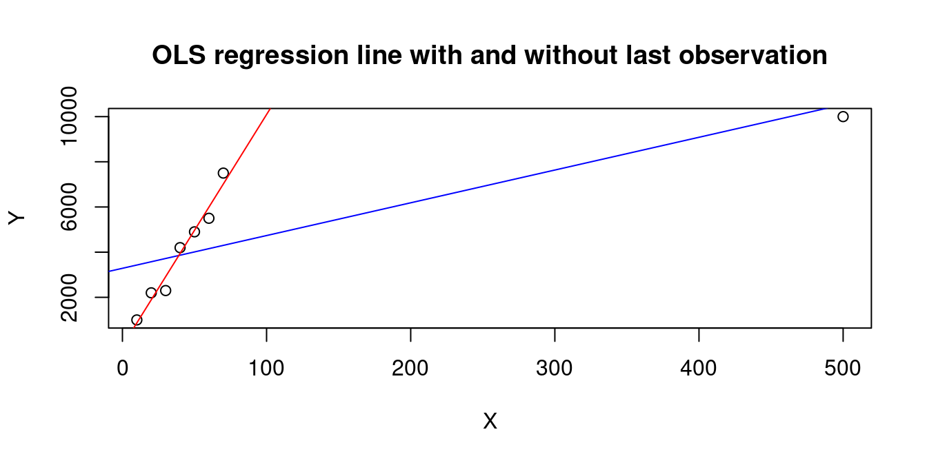
        1         2         3         4         5         6         7         8
0.1657356 0.1569566 0.1492418 0.1425911 0.1370045 0.1324820 0.1290237 0.9869646
The wage and education data is quite balanced and has moderate leverage values:
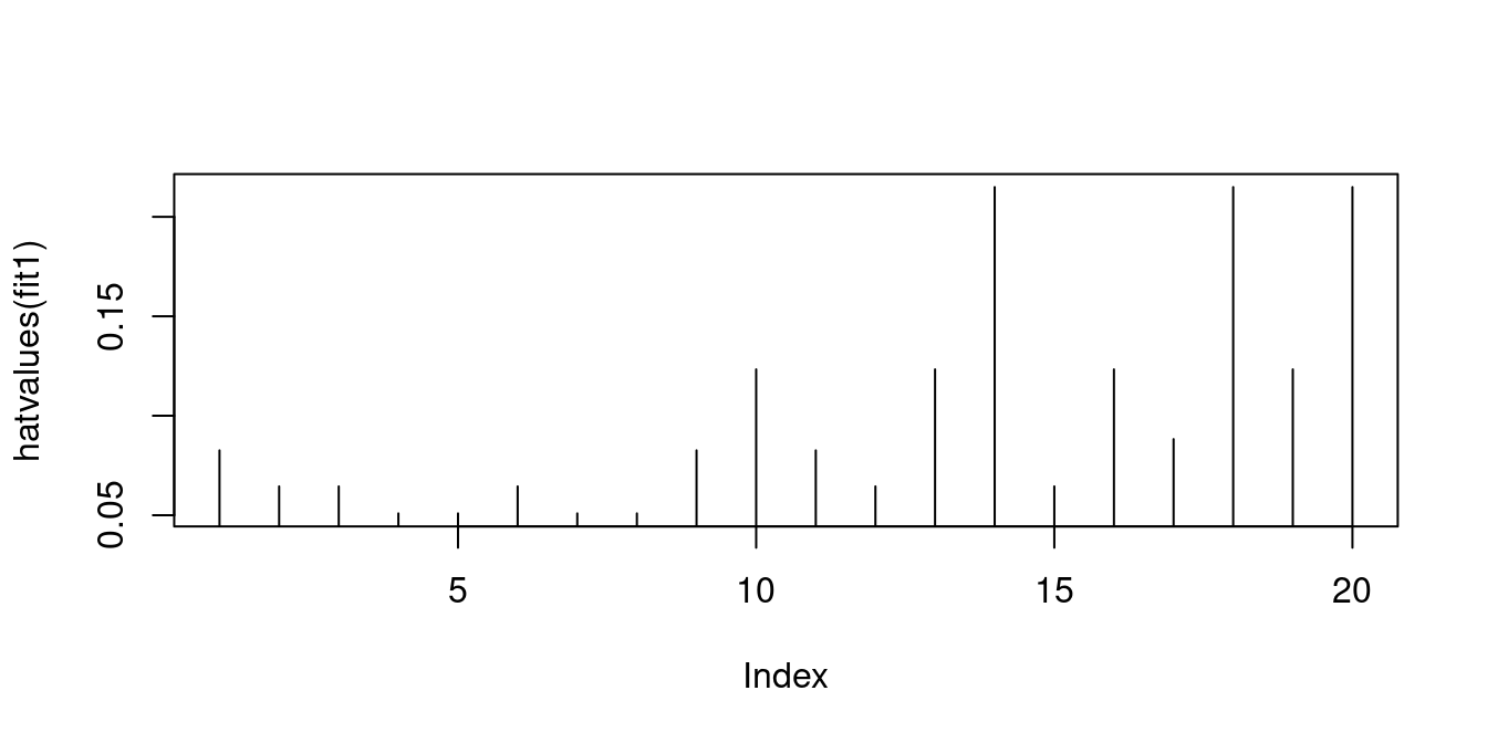
hatvalues(fit1) 1 2 3 4 5 6 7
0.08257919 0.06447964 0.06447964 0.05090498 0.05090498 0.06447964 0.05090498
8 9 10 11 12 13 14
0.05090498 0.08257919 0.12330317 0.08257919 0.06447964 0.12330317 0.21493213
15 16 17 18 19 20
0.06447964 0.12330317 0.08823529 0.21493213 0.12330317 0.21493213 The matrix \boldsymbol M = \boldsymbol I_n - \boldsymbol P = \boldsymbol I_n - \boldsymbol X (\boldsymbol X'\boldsymbol X)^{-1} \boldsymbol X' is the n\times n orthogonal projection matrix that projects any vector from \mathbb{R}^n into the vector space orthogonal to that spanned by \boldsymbol X. It is also called annihilator matrix or residual maker matrix because it maps the vector of response values \boldsymbol Y on the vector of residuals: \boldsymbol M \boldsymbol Y = \widehat{\boldsymbol u}.
The projection matrices \boldsymbol P and \boldsymbol M have some nice properties:
The properties (a)-(c) follow directly from the definitions of \boldsymbol P and \boldsymbol M (try it as an exercise). Using these properties one can show that the residual vector \widehat{\boldsymbol u} is orthogonal to each of the column vectors in \boldsymbol X: \boldsymbol X'\widehat{\boldsymbol u} = \underbrace{\boldsymbol X' \boldsymbol M}_{= \boldsymbol 0_{k \times n}} \boldsymbol Y = \boldsymbol 0_{k \times 1}. \tag{9.5}
Equation 9.5 implies that the residual vector \widehat{\boldsymbol u} is orthogonal to the predicted values vector \boldsymbol{\widehat Y} since \boldsymbol X'\widehat{\boldsymbol u}=\boldsymbol 0_{k \times 1} \quad \Rightarrow\quad \underbrace{\widehat\beta'\boldsymbol X'}_{=\boldsymbol{\widehat Y}'}\widehat{\boldsymbol u}=\underbrace{\widehat\beta'\boldsymbol 0_{k \times 1}}_{=0}.
Hence, OLS produces a decomposition of the dependent variable values into the orthogonal vectors of fitted values and residuals, \boldsymbol Y= \boldsymbol{\widehat Y} + \boldsymbol{\widehat u} = \boldsymbol P \boldsymbol Y + \boldsymbol M \boldsymbol Y, with \boldsymbol{\widehat Y}'\boldsymbol{\widehat u}=0. \tag{9.6}
The first and second sample moments of \boldsymbol Y = (Y_1, \ldots, Y_n)' can be expressed in terms of the sample moments of the fitted values \boldsymbol{\widehat Y} = (\widehat Y_1, \ldots, \widehat Y_n)' and the residuals \boldsymbol{\widehat u} = (\widehat u_1, \ldots, \widehat u_n)'.
The first sample moment is \overline Y = \frac{1}{n} \sum_{i=1}^n Y_i = \frac{1}{n} \bigg( \sum_{i=1}^n \widehat Y_i + \underbrace{\sum_{i=1}^n \widehat u_i}_{= 0} \bigg) = \overline{\widehat Y}, which follows from Equation 9.5 and the fact that the linear regression function contains an intercept. The reason is that, due to the intercept, the first column of \boldsymbol X consists of 1’s, and the first entry of \boldsymbol X'\widehat{\boldsymbol u} is \sum_{i=1}^n \widehat u_i.
The second sample moment is \overline{Y^2} = \frac{1}{n} \sum_{i=1}^n Y_i^2 = \frac{1}{n} \sum_{i=1}^n \widehat Y_i^2 + \frac{2}{n} \underbrace{\sum_{i=1}^n \widehat Y_i \widehat u_i}_{= \boldsymbol{\widehat Y}' \boldsymbol{\widehat u} = 0} + \frac{1}{n} \sum_{i=1}^n \widehat u_i^2 = \overline{\widehat Y^2} + \overline{\widehat u^2}, which follows from Equation 9.6.
The sample variance is \widehat \sigma_Y^2 = \overline{Y^2} - \overline Y^2 = \overline{\widehat Y^2} + \overline{\widehat u^2} - \overline{\widehat Y} = \widehat \sigma_{\widehat Y}^2 + \widehat \sigma_{\widehat u}^2, where \widehat \sigma_{\widehat u}^2 = \overline{\widehat u^2} - \overline{\widehat u}^2 = \overline{\widehat u^2} since \sum_{i=1}^n \widehat u_i = 0 due to the intercept in the regression function.
We obtain the well-known variance decomposition result for OLS regressions:
Analysis-of-variance formula \begin{align*} \underset{\text{total sample variance}}{\frac{1}{n}\sum_{i=1}^n\left(Y_i-\overline{Y}\right)^2}&=&\underset{\text{explained sample variance}}{\frac{1}{n}\sum_{i=1}^n\left(\widehat{Y}_i-\overline{\widehat{Y}}\right)^2}+\underset{\text{unexplained sample variance}}{\frac{1}{n}\sum_{i=1}^n\widehat u_i^2.} \end{align*} Alternatively, we can write \widehat \sigma_Y^2 = \widehat \sigma_{\widehat Y}^2 + \widehat \sigma_{\widehat u}^2 or s_Y^2 = s_{\widehat Y}^2 + s_{\widehat u}^2.
The larger the proportion of the explained sample variance, the better the fit of the OLS regression. This motivates the definition of the so-called R^2 coefficient of determination:
Coefficient of determination
R^2= \frac{\sum_{i=1}^n (\widehat Y_i - \overline{\widehat Y})^2}{\sum_{i=1}^n (Y_i - \overline Y)^2} = 1 - \frac{\sum_{i=1}^n \widehat u_i^2}{\sum_{i=1}^n (Y_i - \overline Y)^2}
R^2 describes the proportion of sample variation in \boldsymbol Y explained by \widehat{\boldsymbol Y}. Obviously, we have that 0\leq R^2\leq 1.
If R^2 = 0, the sample variation in \widehat{\boldsymbol Y} is zero (e.g. if the regression line/surface is horizontally flat). The closer R^2 lies to 1, the better the fit of the OLS regression to the data. If R^2 = 1, the variation in \widehat{\boldsymbol u} is zero, so the OLS regression explains the entire variation in \boldsymbol Y (perfect fit).
A low R^2 does not necessarily mean the regression specification is bad. It just means that there is a high share of unobserved heterogeneity in \boldsymbol Y that is not captured by the regressors \boldsymbol X. A high R^2 does not necessarily mean a good regression specification. It just means that the regression fits the sample well. Too many unnecessary regressors lead to overfitting. If k=n, we have R^2 = 1 even if none of the regressors has an actual influence on the dependent variable.
This brings us to the most commonly criticized drawback of R^2: Additional regressors (relevant or not) always increase the R^2. Here is an example of this problem.
set.seed(123)
n     <- 100                    # Sample size
X     <- runif(n, 0, 10)        # Relevant X variable
X_ir  <- runif(n, 5, 20)        # Irrelevant X variable
extra <- rnorm(n, 0, 10)        # Unobserved additional variable
Y     <- 1 + 5 * X + extra      # Y variable
fit1  <- lm(Y~X)       # Correct OLS regression
fit2   <- lm(Y~X+X_ir)  # OLS regression with X_ir
c(summary(fit1)$r.squared, summary(fit2)$r.squared)
[1] 0.6933407 0.6933606So, R^2 increases here even though X_ir is a completely irrelevant explanatory variable.
## Simulate n-2 additional irrelevant regressors:
X_ir2  <- matrix(runif(n*(n-2), 5, 20),nrow=n)
## use 50 irrelevant regressors:
fit3   <- lm(Y~X+X_ir2[,1:50])
## use all 98 irrelevant regressors:
fit4   <- lm(Y~X+X_ir2)
c(summary(fit3)$r.squared, summary(fit4)$r.squared)
[1] 0.8353157 1.0000000If we add 50 irrelevant regressors, the R^2 increases even further. If we add 98 irrelevant regressors (k=100=n), we obtain a perfect fit with R^2 = 1.
Possible solutions are given by penalized criteria such as the so-called adjusted R-squared or R-bar-squared:
Adjusted R-squared
\overline{R}^2 = 1 - \frac{\frac{1}{n-k}\sum_{i=1}^n \widehat u_i^2}{\frac{1}{n-1}\sum_{i=1}^n (Y_i - \overline Y)^2}
The adjustment is in terms of the degrees of freedom. We lose k degrees of freedom in the OLS regression since we have k regressors (k linear restrictions). We lose one degree of freedom in computing the sample variance due to the sample mean (one linear restriction).
The squareroot of the adjusted sample variance in the numerator of the adjusted R-squared formula is called the standard error of the regression (SER): SER := \sqrt{ \frac{1}{n-k}\sum_{i=1}^n \widehat u_i^2 } = \sqrt{\frac{n}{n-k} \widehat \sigma_{\widehat u}^2}.
An alternative for comparing different regression specifications is the leave-one-out R-squared or R-tilde-squared, which is based on the leave-one-out cross-validation (LOOCV) principle. The i-th leave-one-out OLS coefficient is the OLS coefficient using the sample without the i-th observation: \widehat \beta_{(-i)} = \Big( \sum_{j \neq i} X_j X_j' \Big)^{-1} \sum_{j \neq i} X_j Y_j = (\boldsymbol X' \boldsymbol X - X_i X_i')^{-1} (\boldsymbol X' \boldsymbol Y - X_i Y_i) The i-th leave-one-out predicted value \widetilde Y_i = X_i'\widehat \beta_{(-i)} is an authentic prediction for Y_i since observation Y_i is not used to construct \widetilde Y_i. The leave-one-out residual is \widetilde u_i = Y_i - \widetilde Y_i and obeys the relation \widetilde u_i = \frac{\widehat u_i}{1- h_{ii}}, where h_{ii} = X_i'(\boldsymbol X'\boldsymbol X)^{-1} X_i is the i-th leverage value.
The leave-one-out R-squared is the R-squared using leave-one-out residuals:
Leave-one-out R-squared
\widetilde R^2 = 1 - \frac{\sum_{i=1}^n \widetilde u_i^2}{\sum_{i=1}^n (Y_i - \overline Y)^2} = 1 - \frac{\sum_{i=1}^n \frac{\widehat u_i^2}{(1- h_{ii})^2}}{\sum_{i=1}^n (Y_i - \overline Y)^2}.
Let’s compare the three R-squared versions for various numbers of included regressors.
library(tidyverse)
R2 = function(fit){
  summary(fit)$r.squared
}
AdjR2 = function(fit){
  summary(fit)$adj.r.squared
}
LoocvR2 = function(fit, Y){
  LoocvResid = residuals(fit)/(1-hatvalues(fit))
  1-sum(LoocvResid^2)/sum((Y - mean(Y))^2)
}

## use 90 irrelevant regressors:
fit5   <- lm(Y~X+X_ir2[,1:90])
## use 95 irrelevant regressors:
fit6   <- lm(Y~X+X_ir2[,1:95])

specification = c(0, 1, 50, 90, 95, 98)
Rsquared = sapply(list(fit1, fit2, fit3, fit5, fit6, fit4), R2)
adjRsquared = sapply(list(fit1, fit2, fit3, fit5, fit6, fit4), AdjR2)
LoocvRsquared = sapply(list(fit1, fit2, fit3, fit5, fit6, fit4), LoocvR2, Y=Y)

round(tibble("#irrelevant regressors" = specification, Rsquared, adjRsquared, LoocvRsquared),4) %>% kbl(align = 'c')| #irrelevant regressors | Rsquared | adjRsquared | LoocvRsquared |
|---|---|---|---|
| 0 | 0.6933 | 0.6902 | 0.6799 |
| 1 | 0.6934 | 0.6870 | 0.6738 |
| 50 | 0.8353 | 0.6603 | 0.2681 |
| 90 | 0.9669 | 0.5900 | -5.7026 |
| 95 | 0.9912 | 0.7103 | -30.7321 |
| 98 | 1.0000 | NaN | NaN |
For comparing different OLS regression specifications, the leave-one-out R-squared should be preferred.
The illustrative simulation above shows that the problem of overfitting increases as the number of regressors increases. If k=n we obtain a perfect fit.
par(mfrow=c(1,2))
## k=n=2
Y = c(0.7,-1.0)
X = c(1.9,0.8)
fit1 = lm(Y~X)
plot(X,Y, main="OLS with k=n=2")
abline(fit1)
## k=n=3
# Some given data
Y = c(0.7,-1.0,-0.2)
X_2 = c(1.9,0.8,1.25)
X_3 = c(66, 62, 59)
fit2 = lm(Y ~ X_2 + X_3)
plot3d  <- scatterplot3d(x = X_2, y = X_3, z = Y,
            angle = 33, scale.y = 0.8, pch = 16,
            color ="red",
            xlab = "X_2",
            ylab = "X_3",
            main ="OLS with k=n=3")
plot3d$plane3d(fit2, lty.box = "solid", col=gray(.5), draw_polygon=TRUE)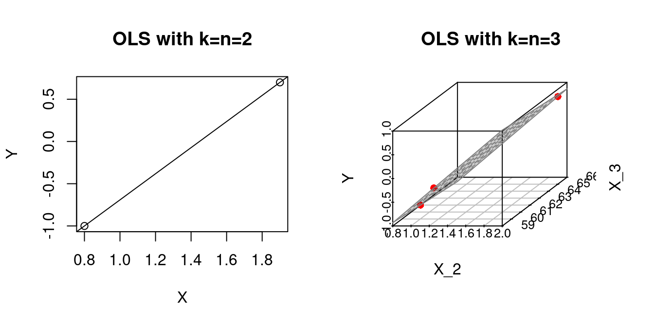
If the number of regressors and observations k=n are higher, we can no longer visualize the OLS fit, but the problem still exists: we have Y_i=\widehat Y_i for all i=1, \ldots n.
For k>n, we cannot compute the OLS regression because \sum_{i=1}^n X_i X_i' = \boldsymbol X' \boldsymbol X is not invertible.
Regression problems with k \approx n or k>n are called high-dimensional regressions. In this case, regularization techniques such as Ridge, Lasso, Elastic-net, or dimension-reduction techniques such as principal components or partial least squares should be used.
OLS should be considered for regression problems with k << n (small k and large n).
The only condition for computing the OLS coefficients is that \sum_{i=1}^n X_i X_i' = \boldsymbol X' \boldsymbol X is invertible.
A necessary condition is that k \leq n, as discussed above.
Another reason the matrix may not be invertible is if two or more regressors are perfectly collinear. Two variables are perfectly collinear if their sample correlation is 1 or -1. We have multicollinearity if one variable is a linear combination of the other variables.
This can happen when the same regressor is included twice or in two different units (e.g., GDP in EUR and USD).
Suppose we include a variable that has the same value for all observations (e.g., a dummy variable where all individuals in the sample belong to the same group). In this case, the variable is collinear with the intercept variable. Including too many dummy variables can lead to the dummy variable trap (see below).
The regressor variables are strictly multicollinear (or perfectly multicollinear) if the regressor matrix does not have full column rank: \text{rank}(\boldsymbol X) < k. It implies \text{rank}(\boldsymbol X' \boldsymbol X) < k, so that the matrix is singular and \widehat \beta cannot be computed.
A related situation is near multicollinearity (often just called multicollinearity). It occurs when two columns of \boldsymbol X have a sample correlation very close to 1 or -1. Then, (\boldsymbol X' \boldsymbol X) is “near singular”, its eigenvalues are very small, and (\boldsymbol X' \boldsymbol X)^{-1} becomes very large, causing numerical problems.
Multicollinearity means that at least one regressor is redundant and can be dropped.
In the following, we consider a simple linear regression model that aims to predict wages in 2015 using gender as the only predictor. We use data provided in the accompanying materials of Stock and Watson’s Introduction to Econometrics textbook. You can download the data stored as an xlsx-file cps_ch3.xlsx HERE.
Let us first prepare the dataset:
## load the 'tidyverse' package
library("tidyverse")
## load the 'readxl' package
library("readxl")

## import the data into R
cps = read_excel(path = "cps_ch3.xlsx")

## Data wrangling
cps_2015 = cps %>% mutate(
    wage   = ahe15,      # rename "ahe15" as "wage"
    gender = fct_recode( # rename factor "a_sex" as "gender"
      as_factor(a_sex),
                "male" = "1",  # rename factor level "1" to "male"
                "female" = "2" # rename factor level "2" to "female"
             )
  ) %>%
  filter(year == 2015) %>%     # Only data from year 2008
  select(wage, gender)         # Select only the variables "wage" and "gender"
The first six lines of the dataset look as follows:
| wage | gender |
|---|---|
| 25.64103 | female |
| 16.02564 | female |
| 33.65817 | male |
| 23.07692 | female |
| 12.98077 | female |
| 11.53846 | male |
Computing the estimation results:
gives
To compute these estimation results, one must assign a numeric 0/1 coding to the factor levels male and female of the factor variable gender. To see the numeric values used by R, one can take a look at model.matrix(lm_obj):
X = model.matrix(lm_obj) # this is the internally used X-matrix
X[1:6,]
(Intercept) genderfemale
1 1 1
2 1 1
3 1 0
4 1 1
5 1 1
6 1 0cps_2015$gender[1:6][1] female female male female female male
Levels: male femaleThus, R internally codes female subjects by 1 and male subjects by 0, such that
\widehat\beta_1 + \widehat\beta_2 X_{i,gender}=\left\{\begin{array}{ll}\widehat\beta_1&\text{ if }X_{i,gender}=\text{male}\\\widehat\beta_1 + \widehat\beta_2&\text{ if }X_{i,gender}=\text{female}\end{array} \right.
Interpretation:
Above, we used R’s internal handling of factor variables, which you should always do. However, if you construct a dummy variable for each of the levels of a factor, you may fall into the dummy variable trap:
Computing the OLS coefficients “by hand” yields
Error in solve.default(X %*% t(X)) :
  system is exactly singular
An error message! We fell into the dummy variable trap!
The estimation result is not computable since (\boldsymbol X' \boldsymbol X) is not invertible due to the perfect multicollinearity between the intercept and the two dummy variablesX_female and X_male
X_1 = X_female + X_male
which violates the invertibility condition (no perfect multicollinearity).
Solution: Use one dummy variable less than factor levels. I.e., in this example, you can drop X_female or X_male.
## New model matrix after dropping X_male:
X        <- cbind(X_1, X_female)

## Computing the estimator
beta_hat <- solve(t(X) %*% X) %*% t(X) %*% Y
beta_hat
[,1]
X_1 28.05536
X_female -5.01638This gives the same result as computed by R’s lm() function using the factor variable gender:
f(X_i) = 28.055 -5.016 X_{i,female}.
An intercept is not necessarily required for the OLS method. In this case, the first column of the regressor matrix \boldsymbol X does not contain 1’s. An alternative to solve the dummy variable trap is to drop the intercept:
## Write -1 to drop the intercept
lm_obj2 = lm(Y~X_female+X_male-1)
coefficients(lm_obj2)
X_female X_male
23.03898 28.05536 The fitted regression function is f(X_i) = 23.039 X_{i,female} + 28.055 X_{i,male}.
Notice the different interpretations of the OLS coefficients!