[1] 1.006031 1.9842177 Hypothesis Testing
7.1 Statistical hypotheses
A statistical hypothesis is a statement about the population distribution. For instance, we might be interested in the hypothesis that the mean \mu = E[Y] of a random variable Y is equal to some value \mu_0 or whether it is unequal to that value.
In hypothesis testing, we divide the parameter space of interest into a null hypothesis and an alternative hypothesis, for instance \underbrace{H_0:\mu = \mu_0}_{ \text{null hypothesis} } \quad \text{vs.} \quad \underbrace{H_1:\mu \neq \mu_0,}_{ \text{alternative hypothesis} } \tag{7.1} or, more generally, H_0: \theta = \theta_0. In practice, two-sided alternatives are more common, i.e. H_1: \theta \neq \theta_0, but one-sided alternatives are also possible, i.e. H_1: \theta > \theta_0 (right-sided) or H_1: \theta < \theta_0 (left-sided).
We are interested in testing H_0 against H_1. The idea of hypothesis testing is to construct a statistic T_0 (test statistic) for which the sampling distribution under H_0 (null distribution) is known, and for which the distribution under H_1 differs from the null distribution (i.e., the null distribution is informative about H_1).
If the observed value of T_0 takes a value that is likely to occur under the null distribution, we deduce that there is no evidence against H_0, and consequently we do not reject H_0 (we accept H_0). If the observed value of T_0 takes a value that is unlikely to occur under the null distribution, we deduce that there is evidence against H_0, and consequently, we reject H_0 in favor of H_1. “Unlikely” means that its occurrence has only a small probability \alpha. The value \alpha is called the significance level and must be selected by the researcher. It is conventional to use the values \alpha = 0.1, \alpha=0.05, or \alpha = 0.01, but it is not a hard rule.
A hypothesis test with significance level \alpha is a decision rule defined by a rejection region I_1 and an acceptance region I_0 = I_1^c so that we \begin{align*} \text{do not reject} \ H_0 \quad \text{if} \ &T_0 \in I_0, \\ \text{reject} \ H_0 \quad \text{if} \ &T_0 \in I_1. \end{align*} The rejection region is defined such that a false rejection occurs with probability \alpha, i.e. P( \underbrace{T_0 \in I_1}_{\text{reject}} \mid H_0 \ \text{is true}) = \alpha, \tag{7.2} where P(\cdot \mid H_0 \ \text{is true}) denotes the probability function of the null distribution.
A test that satisfies Equation 7.2 is called a size-\alpha-test. The type I error is the probability of falsely rejecting H_0 and equals \alpha for a size-\alpha-test. The type II error is the probability of falsely accepting H_0 and depends on the sample size n and the unknown parameter value \theta under H_1. Typically, the further \theta is from \theta_0, and the larger the sample size n, the smaller the type II error.
The probability of a type I error is also called the size of a test: P( \text{reject} \ H_0 \mid H_0 \ \text{is true}). The power of a test is the complementary probability of a type II error: P( \text{reject} \ H_0 \mid H_1 \ \text{is true}) = 1 - P( \text{accept} \ H_0 \mid H_1 \ \text{is true}). A hypothesis test is consistent for H_1 if the power tends to 1 as n tends to infinity for any parameter value under the alternative.
| Accept H_0 | Reject H_0 | |
| H_0 is true | correct decision | type I error |
| H_1 is true | type II error | correct decision |
In many cases, the probability distribution of T_0 under H_0 is known only asymptotically. Then, the rejection region must be defined such that \lim_{n \to \infty} P( T_0 \in I_1 \mid H_0 \ \text{is true}) = \alpha. We call this test an asymptotic size-\alpha-test.
The decision “accept H_0” does not mean that H_0 is true. Since the probability of a type II error is unknown in practice, it is more accurate to say that we “fail to reject H_0” instead of “accept H_0”. The power of a consistent test tends to 1 as n increases, so type II errors typically occur if the sample size is too small. Therefore, to interpret a “fail to reject H_0”, we have to consider whether our sample size is relatively small or rather large.
7.2 t-Test for the mean
For tests concerning the population mean, we can use the standardized sample mean, where we replace the sampling standard deviation with a standard error. The classical t-statistic or t-ratio for H_0: \mu = \mu_0 is T_0 := \frac{\overline Y - \mu_0}{se(\overline Y)} = \frac{\overline Y - \mu_0}{s_Y/\sqrt{n}}.
To construct a test of size \alpha based on T_0, we first have to study the null distribution of T_0.
7.2.1 The normal i.i.d. case
Let’s start with the restrictive case that the sample \{Y_1, \ldots, Y_n\} is i.i.d. and normally distributed with Y_i \sim \mathcal N(\mu, \sigma^2), and recall from the previous section that, in this case, \frac{\overline Y - \mu}{s_Y/\sqrt{n}} \sim \mathcal t_{n-1} \tag{7.3} for any fixed sample size n.
If the null hypothesis H_0: \mu = \mu_0 is true, the t-ratio satisfies T_0 := \frac{\overline Y - \mu_0}{s_Y/\sqrt{n}} = \frac{\overline Y - \mu}{s_Y/\sqrt{n}} \sim \mathcal t_{n-1}, i.e., the null distribution of T_0 is t_{n-1}.
Under the alternative hypothesis H_1: \mu \neq \mu_0, we have T_0 = \frac{\overline Y - \mu_0}{s_Y/\sqrt{n}} = \underbrace{\frac{\overline Y - \mu}{s_Y/\sqrt{n}}}_{\sim t_{n-1}} + \underbrace{\frac{\mu - \mu_0}{s_Y/\sqrt{n}}}_{\neq 0} \nsim \mathcal t_{n-1}. The second term (\mu - \mu_0)/(s_Y/\sqrt{n}) diverges as n increases. It becomes to + \infty or - \infty depending on whether \mu - \mu_0 is positive or negative. The distribution under H_1 differs from the null distribution. The null distribution is therefore informative about H_1.
The idea is to compute T_0 for the given sample and check whether its value fits better to the null distribution or the alternative distribution of T_0. More precisely, we define a decision rule so that Equation 7.2 is satisfied. Since the null distribution has mean zero and some finite variance and the alternative distribution diverges to +\infty or -\infty, it makes sense to accept H_0 if T_0 is close to zero and reject if it takes large positive or negative values.
We define the acceptance and rejection regions I_0 and I_1 by fixing a critical value c with the following decision rule: \begin{align*} \text{do not reject} \ H_0 \ \text{if} \ &|T_0| \leq c, \\ \text{reject} \ H_0 \ \text{if} \ &|T_0| > c. \end{align*}
Let F_0(a) = P(T_0 \leq a \mid H_0 \ \text{is true}) be the CDF of the null distribution, i.e., F_0 is the CDF of t_{n-1}. To determine a critical value c that satisfies Equation 7.2, first note that c must be positive (otherwise, we would always reject). Moreover, \begin{align*} P(\text{reject} \ H_0 \mid H_0 \ \text{is true}) &= P(|T_0| > c \mid H_0 \ \text{is true}) \\ &= P\big(\{ T_0 < -c \} \cup \{ T_0 > c \} \mid H_0 \ \text{is true}\big) \\ &= P(T_0 < -c \mid H_0 \ \text{is true}) + P(T_0 > c \mid H_0 \ \text{is true}) \\ &= F_0(-c) + (1 - F_0(c)) \\ &= 2(1 - F_0(c)), \end{align*} where the last step follows from F_0(-c) = 1-F_0(c) due to the fact that t_{n-1} is a symmetric distribution. Finally, setting equal to \alpha and solving for c yields \begin{align*} && 2(1 - F_0(c)) &= \alpha \\ \Leftrightarrow&& \qquad \qquad F_0(c) &= 1-\frac{\alpha}{2} \\ \Leftrightarrow&& \qquad \qquad c &= F_0^{-1}(1-\tfrac{\alpha}{2}) \\ \Leftrightarrow&& \qquad \qquad c &= t_{(n-1;1-\frac{\alpha}{2})}, \end{align*} which is the 1-\alpha/2 quantile of the t-distribution with n-1 degrees of freedom.
Hence, we reject H_0 if |T_0| exceeds t_{(n-1;1-\frac{\alpha}{2})}. Equivalently, H_0 is rejected if \mu_0 is not element of the (1-\alpha) confidence interval Equation 6.9.
7.2.2 The non-normal i.i.d. case
If \{ Y_1, \ldots, Y_n \} is i.i.d. and non-normal, the CLT implies that Equation 7.3 is replaced by the asymptotic result \frac{\overline Y - \mu}{s_Y/\sqrt{n}} \overset{D}{\rightarrow} \mathcal N(0,1) as n \to \infty. Therefore, an asymptotic size-\alpha-test for the hypotheses in Equation 7.1 is defined by the following decision rule: \begin{align*} \text{do not reject} \ H_0 \quad \text{if} \ &|T_0| \leq z_{(1-\frac{\alpha}{2})}, \\ \text{reject} \ H_0 \quad \text{if} \ &|T_0| > z_{(1-\frac{\alpha}{2})}. \end{align*}
Alternatively, since t_{n-1} \overset{D}{\rightarrow} \mathcal N(0,1) and therefore \lim_{n \to \infty} t_{(n-1;1-\frac{\alpha}{2})} = z_{(1-\frac{\alpha}{2})}, we may also use t-quantiles and apply the decision rule \begin{align*} \text{do not reject} \ H_0 \quad \text{if} \ &|T_0| \leq t_{(n-1;1-\frac{\alpha}{2})}, \\ \text{reject} \ H_0 \quad \text{if} \ &|T_0| > t_{(n-1;1-\frac{\alpha}{2})}. \end{align*}
Let’s test the hypothesis that H_0: E(wage) = 16 against H_1: E(wage) \neq 16.
The test statistic T_0 = 1.01 is in absolute value smaller than the critical value c = 1.98 at the 5% significance level. Therefore, we do not reject H_0. Alternatively, we can use the t.test(wg, mu=16) function (see below). If we use the normal quantile, we have the critical value c = 1.96, which yields the same test decision.
7.2.3 The time series case
If \{ Y_1, \ldots, Y_n \} is a stationary short-memory time series, classical standard errors are not valid since \frac{\overline Y - \mu}{s_Y/\sqrt{n}} \overset{D}{\rightarrow} \mathcal N\Big(0,\frac{\omega^2}{\sigma^2}\Big). We may use Newey-West standard errors se_{nw}(\overline Y), which yield \frac{\overline Y - \mu}{\widehat \omega_{nw}/\sqrt{n}} \overset{D}{\rightarrow} \mathcal N(0,1). The autocorrelation robust t-ratio for H_0: \mu=\mu_0 is given by T_{0,AC} = \frac{\overline Y - \mu_0}{\widehat \omega_{nw}/\sqrt{n}}, and an asymptotic test of size \alpha is given by the decision rule \begin{align*} \text{do not reject} \ H_0 \quad \text{if} \ &|T_{0,AC}| \leq z_{(1-\frac{\alpha}{2})}, \\ \text{reject} \ H_0 \quad \text{if} \ &|T_{0,AC}| > z_{(1-\frac{\alpha}{2})}. \end{align*} Alternatively, t-quantiles may be used.
Let’s test the hypothesis that H_0: E(gdpgrowth) = 4 against H_1: E(gdpgrowth) \neq 4.
library(sandwich)
seNW = sqrt(NeweyWest(lm(gdp~1)))
tratio = (mean(gdp)-4)/seNW
crit = qnorm(0.975)
c(tratio, crit)
[1] -2.250481 1.959964We reject H_0 since |T_{0,AC}| = 2.25 > 1.96. There is no statistical evidence that the mean GDP growth is 4.
7.3 The p-value
The p-value is a criterion to reach the t-test decision conveniently: \begin{align*} \text{reject} \ H_0 \quad &\text{if p-value} < \alpha \\ \text{do not reject} \ H_0 \quad &\text{if p-value} \geq \alpha \end{align*}
Formally, the p-value of a two-sided t-test is defined as p\text{-value} = P( | \widetilde T| > |T_0| \mid H_0 \ \text{is true}), where \widetilde T is a random variable with the null distribution, i.e. \widetilde T\sim t_{n-1}. The p-value is the probability that a null-distributed random variable produces values at least as extreme as the test statistic T_0 produced for your sample. We can express the p-value also using the CDF F_0 of the null distribution: \begin{align*} p\text{-value} &= P(| \widetilde T| > |T_0| \mid H_0 \ \text{is true}) \\ &= 1 - P(|\widetilde T| \leq |T_0| \mid H_0 \ \text{is true}) \\ &= 1 - F_0(|T_0|) + F_0(-|T_0|) \\ &= 2(1 - F_0(|T_0|)). \end{align*}
Make no mistake, the p-value is not the probability that H_0 is true! It is a measure of how likely it is that the observed test statistic comes from a sample that has been drawn from the null distribution.
To compute the p-value by hand, we have to insert the t-statistic into the CDF of the null distribution:
tratio = (mean(wg)-16)/(sd(wg)/sqrt(length(wg)))
df = length(wg)-1
2*(1-pt(abs(tratio), df)) ## p-value
[1] 0.3168532The t.test() function provides a summary of all relevant statistics for inference on the mean: the sample mean, a 95%-confidence interval, the t-statistic for a specified null hypothesis, and the corresponding p-value:
t.test(wg, mu=16)
    One Sample t-test

data:  wg
t = 1.006, df = 99, p-value = 0.3169
alternative hypothesis: true mean is not equal to 16
95 percent confidence interval:
 14.97362 19.13758
sample estimates:
mean of x
  17.0556
7.4 Power function
Consider an i.i.d. sample \{Y_1, \ldots, Y_n\} from a distribution with mean \mu and variance \sigma^2. The power function of the two-sided t-test for H_0: \mu = \mu_0 is defined as \pi(\mu, \sigma^2, n) = P(\text{reject} \ H_0) = P(|T_0| > c), where c = z_{(1-\frac{\alpha}{2})} (or a corresponding t-quantile).
For \mu = \mu_0 (i.e., H_0 is true), \pi(\mu_0, \sigma^2, n) corresponds to the size and the probability of a type I error. For \mu \neq \mu_0 (i.e., H_1 is true), we have \pi(\mu, \sigma^2, n) = (1 - P(\text{type II error})).
Consider for simplicity the test for a zero mean, i.e., \mu_0 = 0, and suppose the true mean is different, i.e., \mu \neq 0. The test statistic is T_0 = \frac{\overline Y - 0}{se(\overline Y)} = \frac{ \overline Y}{s_Y / \sqrt n}, and we have T_0 - \frac{\sqrt n \mu}{s_Y} = \frac{ \overline Y - \mu}{s_Y / \sqrt n} \overset{D}{\to} \mathcal N(0,1), which implies that P(T_0 \leq c) = P\bigg(\frac{\overline Y - \mu}{s_Y/\sqrt n} \leq c - \frac{\sqrt n \mu}{s_Y}\bigg) \approx \Phi(c-\sqrt n \mu / \sigma ). In the last step, we also used that s_Y^2 is consistent for \sigma^2. The power function then becomes \begin{align*} \pi(\mu, \sigma^2, n) &= P(|T_0| > c) \\ &= 1 - P(-c \leq T_0 \leq c) \\ & 1 - P(T_0 \leq c) + P(T_0 \leq -c) \\ &\approx 1 - \Phi(c -\sqrt n \mu / \sigma ) + \Phi(-c-\sqrt n \mu / \sigma ). \end{align*}
Below you find a plot of the power curve for different values of \sqrt n \mu / \sigma and significance levels:
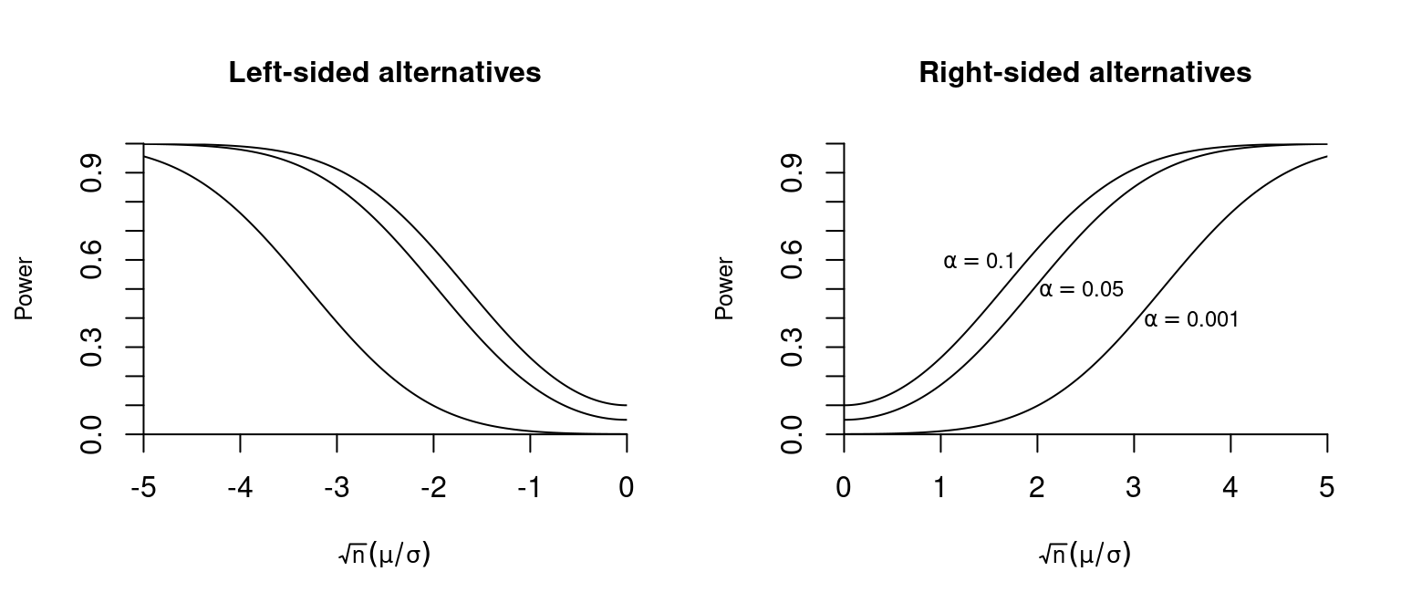
Since (\pm c -\sqrt n \mu / \sigma) \to \infty as n \to \infty, we have, for \mu > 0, 1 - \underbrace{\Phi(c -\sqrt n \mu / \sigma )}_{\to 0} + \underbrace{\Phi(-c-\sqrt n \mu / \sigma )}_{\to 0} \to 1. Similarly, for alternatives \mu < 0, we have 1 - \underbrace{\Phi(c -\sqrt n \mu / \sigma )}_{\to 1} + \underbrace{\Phi(-c-\sqrt n \mu / \sigma )}_{\to 1} \to 1. Hence, the test is consistent for any alternative \mu \neq 0.
7.5 One-sided t-test
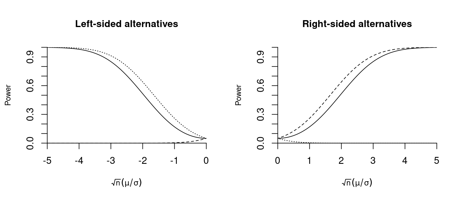
The two-sided t-test is a powerful test for any alternative \mu \neq \mu_0, but it is not the uniformly most powerful test. For a right-sided alternative \mu > 0, the right-sided t-test has a higher power. The following decision rule defines it: \begin{align*} \text{do not reject} \ H_0 \quad \text{if} \ & T_0 \leq z_{(1-\alpha)}, \\ \text{reject} \ H_0 \quad \text{if} \ & T_0 > z_{(1-\alpha)}. \end{align*}
The power function is \pi(\mu, \sigma^2, n) = P(T_0 > z_{(1-\alpha)}) \approx 1 - \Phi\big( z_{(1-\alpha)} - \sqrt n \mu / \sigma \big), which is larger than the power function of the two-sided test for right-sided alternatives. For left-sided alternatives, the right-sided test has no power. The size is \pi(0, \sigma^2, n) \approx 1 - \Phi\big( z_{(1-\alpha)} \big) = \alpha.
Similarly, the left-sided t-test is defined by the decision rule \begin{align*} \text{do not reject} \ H_0 \quad \text{if} \ & T_0 \geq -z_{(1-\alpha)}, \\ \text{reject} \ H_0 \quad \text{if} \ & T_0 < -z_{(1-\alpha)}. \end{align*} Its power function is \pi(\mu, \sigma^2, n) = P(T_0 < -z_{(1-\alpha)}) \approx \Phi\big( -z_{(1-\alpha)} - \sqrt n \mu / \sigma \big), where the size is \pi(\mu, \sigma^2, n) \approx \Phi( -z_{(1-\alpha)}) = \alpha. It has a higher power for left-sided alternatives than the two-sided test but has no power for right-sided alternatives.
It can be shown that, for the fixed simple alternative \mu > \mu_0, the right-sided t-test is the test with the highest possible power, and for an alternative of the form \mu < \mu_0, the left-sided t-test has the greatest power. It is a result of the Neyman-Pearson lemma, which states that no test exists for a simple hypothesis with greater power than a likelihood-ratio test. It can also be shown that the one-sided t-test is equivalent to the likelihood ratio test for the alternative of interest.
Note that the direction of testing must be specified in advance, which is not always practical. The two-sided t-test has slightly less power but is more common in practice because it has power against both right- and left-sided alternatives.
Below, you will find an interactive shiny app for the right-sided z-test. A z-test is a t-test with known variance, where s_Y is replaced by \sigma in the test statistic (i.e., the two tests are asymptotically equivalent).
7.6 Testing for autocorrelation
Consider a stationary time series \{Y_1, \ldots, Y_n\} with order \tau autocorrelation function \rho(\tau) and finite fourth moments (E[Y_i^4] < \infty). We have the following limit theorem for the sample autocorrelation function under H_0: \rho(\tau) = 0: \sqrt n \big(\widehat \rho(\tau) - \rho(\tau)\big) \overset{D}{\to} \mathcal N(0,1).
To test the null hypothesis H_0: \rho(\tau) = 0 for some fixed \tau, consider the test statistic T_0 = \frac{\widehat \rho(\tau)}{1/\sqrt n}, which is standard normal in the limit under H_0. Therefore, a simple test for zero order \tau autocorrelation is given by the decision rule \begin{align*} \text{do not reject} \ H_0 \quad \text{if} \ & |T_0| \leq z_{(1-\frac{\alpha}{2})}, \\ \text{reject} \ H_0 \quad \text{if} \ & |T_0| > z_{(1-\frac{\alpha}{2})}. \end{align*} Equivalently, we reject H_0 if \widehat \rho(\tau) lies outside \pm z_{(1-\frac{\alpha}{2})}/\sqrt n.
The interval [-z_{(1-\frac{\alpha}{2})}/\sqrt n; \ z_{(1-\frac{\alpha}{2})}/\sqrt n] for \alpha = 0.05 is indicated in the ACF plot in R by blue dashed lines. Hence, GDP growth has significant autocorrelation at lag 3 but not at lag 4:
acf(gdp)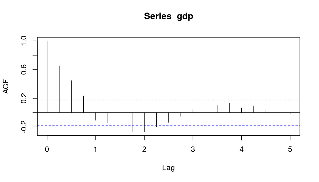
7.7 Additional reading
- Stock and Watson (2019), Sections 3
- Hansen (2022a), Section 13