mean(wg)[1] 17.0556mean(edu)[1] 14.95A parameter \theta is a feature (function) of the population distribution F. We often use Greek letters for parameters. The expectation, variance, correlation, autocorrelation, and regression coefficients are parameters.
A statistic is a function of a sample \{X_i, \ i=1, \ldots, n\}. An estimator \widehat \theta for \theta is a statistic intended as a guess about \theta. It is a function of the random vectors X_1, \ldots, X_n and, therefore, a random variable. When an estimator \widehat \theta is calculated in a specific realized sample, we call \widehat \theta an estimate.
Consider the moments of some bivariate random variable (Y,Z). The sample moments are the corresponding average values in the sample \{(Y_i, Z_i), \ i=1, \ldots,n \}:
| population moment | sample moment |
|---|---|
| E[Y] | \displaystyle \frac{1}{n} \sum_{i=1}^n Y_i |
| E[Z] | \displaystyle \frac{1}{n} \sum_{i=1}^n Z_i |
| E[Y^2] | \displaystyle \frac{1}{n} \sum_{i=1}^n Y_i^2 |
| E[Z^2] | \displaystyle \frac{1}{n} \sum_{i=1}^n Z_i^2 |
| E[YZ] | \displaystyle \frac{1}{n} \sum_{i=1}^n Y_i Z_i |
Many parameters of interest can be expressed as a function of the population moments. A common estimation approach is the moment estimator, where the population moments are replaced by their corresponding sample moments.
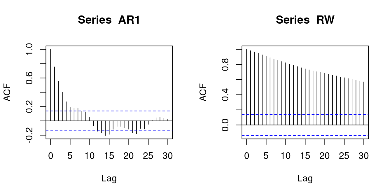
The vectors wg, edu, gdp, and infl contain the datasets on wage, education, GDP growth, and inflation from the previous section, and AR1 and RW are the simulated AR(1) and random walk series.
Mean and sample mean \begin{align*}
\mu_Y &= E[Y] \\
\overline Y &= \frac{1}{n} \sum_{i=1}^n Y_i
\end{align*} If Y is your sample stored in a vector, the R command for the sample mean is: mean(Y) or sum(Y)/length(Y)
Variance and sample variance \begin{align*}
\sigma_Y^2 &= Var[Y] = E[(Y - E[Y]^2)] = E[Y^2] - E[Y]^2 \\
\widehat \sigma_Y^2 &= \frac{1}{n} \sum_{i=1}^n (Y_i - \overline Y)^2 = \frac{1}{n} \sum_{i=1}^n Y_i^2 - \overline Y^2
\end{align*} Sample variance in R: mean((Y-mean(Y))^2).
Note that the command var(Y) returns the bias-corrected sample variance, which slightly deviates from the sample variance:
s_Y^2 = \frac{1}{n-1} \sum_{i=1}^n (Y_i - \overline Y)^2 = \frac{n}{n-1} \widehat \sigma_Y^2.
\tag{5.1} It is common to report the bias-corrected version s_Y^2 instead of \widehat \sigma_Y^2, as it has slightly better properties (see Section 5.6 below). However, this does not matter for large samples since n/(n-1) \to 1 as n \to \infty.
[1] 108.9961[1] 7.4875var(wg) ## bias-corrected sample variance[1] 110.0971var(edu)[1] 7.563131Standard deviation and sample standard deviation \begin{align*}
\sigma_Y &= sd(Y) = \sqrt{Var[Y]} \\
\widehat \sigma_Y &= \sqrt{\widehat \sigma_Y^2}
\end{align*} Sample standard deviation in R: sqrt(mean((Y-mean(Y))^2)).
Note that the command sd(Y) returns the bias-corrected sample standard deviation, which is the square root of Equation 5.1, and slightly deviates from \widehat \sigma_Y. Similarly to the bias-corrected variance, the bias-corrected standard deviation s_Y is typically reported instead of \widehat \sigma_Y.
Skewness and sample skewness \begin{align*}
skew(Y) &= \frac{E[(Y-E[Y])^3}{sd(Y)^3} \\
\widehat{skew} &= \frac{\frac{1}{n} \sum_{i=1}^n (Y_i - \overline Y)^3}{\widehat \sigma_Y^3}
\end{align*} Sample skewness in R: mean((Y-mean(Y))^3)/sqrt(mean((Y-mean(Y))^2))^3. Alternatively, the command skewness(Y) of the package moments can be used.
Kurtosis and sample kurtosis \begin{align*}
kurt(Y) &= \frac{E[(Y-E[Y])^4}{sd(Y)^4} \\
\widehat{kurt} &= \frac{\frac{1}{n} \sum_{i=1}^n (Y_i - \overline Y)^4}{\widehat \sigma_Y^4}
\end{align*} Sample skewness in R: mean((Y-mean(Y))^4)/mean((Y-mean(Y))^2)^2. Alternatively, the command kurtosis(Y) of the package moments can be used.
Covariance and sample covariance \begin{align*}
\sigma_{YZ} &= Cov(Y,Z) = E[(Y - E[Y])(Z-E[Z])] = E[YZ] - E[Y] E[Z] \\
\widehat \sigma_{YZ} &= \frac{1}{n} \sum_{i=1}^n (Y_i - \overline Y) (Z_i - \overline Z) = \frac{1}{n} \sum_{i=1}^n Y_i Z_i - \overline Y \cdot \overline Z
\end{align*} Sample covariance in R: mean((Y-mean(Y))*(Z-mean(Z))). Note that cov(Y,Z) returns the bias-corrected sample covariance s_{YZ} = n/(n-1) \cdot \widehat \sigma_{YZ}.
Correlation and sample correlation \begin{align*}
\rho_{YZ} &= \frac{Cov(Y,Z)}{sd(Y)sd(Z)} \\
\widehat \rho_{YZ} &= \frac{\widehat \sigma_{YZ}}{\widehat \sigma_Y \widehat \sigma_Z}
\end{align*} Sample correlation in R: cor(Y,Z).
cor(wg, edu)[1] 0.3651786Autocovariance and sample autocovariance \begin{align*}
\gamma(\tau) &= Cov(Y_t, Y_{t-\tau}) = E[(Y_t - \mu_Y)(Y_{t-\tau} - \mu_Y)] \\
\widehat \gamma(\tau) &= \frac{1}{n} \sum_{i=\tau+1}^n (Y_i - \overline Y) (Y_{i-\tau} - \overline Y)
\end{align*} Sample autocovariances in R: acf(Y, type = "covariance", plot = FALSE). Note that acf(Y, type = "covariance") returns a plot of the sample autocovariance function.
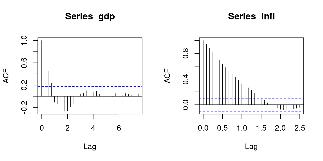
acf(gdp, type = "covariance", plot = FALSE)
Autocovariances of series 'gdp', by lag

   0.00    0.25    0.50    0.75    1.00    1.25    1.50    1.75    2.00    2.25
 6.6348  4.2772  2.9628  1.5468 -0.7084 -0.9210 -1.3339 -1.7877 -1.7673 -1.2969
   2.50    2.75    3.00    3.25    3.50    3.75    4.00    4.25    4.50    4.75
-0.9022 -0.3446  0.2861  0.3126  0.6607  0.8516  0.4438  0.5634  0.2310 -0.1504
   5.00
-0.0926 acf(infl, type = "covariance", plot = FALSE)
Autocovariances of series 'infl', by lag

  0.0000   0.0833   0.1667   0.2500   0.3333   0.4167   0.5000   0.5833
 2.25940  2.12625  1.99568  1.85704  1.71710  1.56860  1.42454  1.30920
  0.6667   0.7500   0.8333   0.9167   1.0000   1.0833   1.1667   1.2500
 1.19518  1.07702  0.96450  0.85573  0.73584  0.66869  0.59613  0.50944
  1.3333   1.4167   1.5000   1.5833   1.6667   1.7500   1.8333   1.9167
 0.41708  0.32785  0.24573  0.15681  0.06751  0.00289 -0.06278 -0.11801
  2.0000   2.0833
-0.15911 -0.17548
Autocorrelation and sample autocorrelation \begin{align*}
\rho(\tau) &= \frac{\gamma(\tau)}{\gamma(0)} = \frac{Cov(Y_t, Y_{t-\tau})}{Var[Y_t]} \\
\widehat \rho(\tau) &= \frac{\widehat \gamma(\tau)}{\widehat \gamma(0)}
\end{align*} Sample autocorrelations in R: acf(Y, plot = FALSE). Note that acf(Y) returns a plot of the sample autocorrelation function.
Note that the lags on the x-axis are measured in yeas, where gdp is quarterly data and infl is monthly data.
The ACF plots indicate the dynamic structure of the time series and whether they can be regarded as a stationary and short-memory time series. The ACF of gdp tends to zero quickly, similar to the ACF of the AR1. They can be treated as stationary and short-memory time series. The ACF of infl tends to zero slowly, indicating a high persistence, so the short-memory condition may not be satisfied. The ACF of RW does not tend to zero. It is a nonstationary time series.
Good estimators get closer and closer to the true parameter being estimated as the sample size n increases, eventually returning the true parameter value in a hypothetically infinitely large sample. This property is called consistency.
Consistency
An estimator \widehat \theta is consistent for a true parameter value \theta if \begin{align*} \lim_{n \to \infty} P(|\widehat \theta - \theta| > \epsilon) = 0 \qquad \text{for any} \ \epsilon > 0, \end{align*} or, equivalently, if P(|\widehat \theta - \theta| \leq \epsilon) \to 1 as n \to \infty.
If \widehat \theta is consistent for \theta, we say that \widehat \theta converges in probability to \theta. A common notation for convergence in probability is the probability limit: \begin{align*} \plim_{n \to \infty} \widehat \theta = \theta, \quad \text{or} \quad \widehat \theta \overset{p} \to \theta. \end{align*}
Since an estimator \widehat \theta is usually a continuous random variable, it will almost never reach exactly the true parameter value: P(\widehat \theta = \theta) = 0. However, the larger the sample size, the higher should be the probability that \widehat \theta is close to the true value \theta. Consistency means that, if we fix some small precision value \epsilon > 0, then, P(|\widehat \theta - \theta| \leq \epsilon) = P( \theta - \epsilon \leq \widehat \theta \leq \theta + \epsilon) should increase in the sample size n and eventually reach 1.
An estimator is called inconsistent if it is not consistent. An inconsistent estimator is practically useless.
To show whether an estimator is consistent, we can check the sufficient condition for consistency:
Sufficient condition for consistency
The mean squared error (MSE) of an estimator \widehat \theta for some parameter \theta is defined as mse(\widehat \theta) = E[(\widehat \theta - \theta)^2]. If mse(\widehat \theta) tends to 0 as n \to \infty, then \widehat \theta is consistent for \theta.
The sufficient condition is a direct application of Markov’s inequality, which states that, for any random variable Z, any \epsilon > 0, and any r \in \mathbb N, we have P(|Z| \geq \epsilon) \leq \frac{E[|Z|^r]}{\epsilon^r}. Consequently, with Z = \widehat \theta - \theta, and r = 2, we get \begin{align*} P(|\widehat \theta - \theta| > \epsilon) \leq \frac{E[|\widehat \theta - \theta|^2]}{\epsilon^2} = \frac{mse(\widehat \theta)}{\epsilon^2}. \end{align*} Then, mse(\widehat \theta) \to 0 is a sufficient condition for consistency since it implies P(|\widehat \theta - \theta| > \epsilon) \to 0 due to the inequality in the formula above.
The mean square error of any estimator \widehat \theta can be decomposed into two additive terms, mse(\widehat \theta) = var[\widehat \theta] + bias[\widehat \theta]^2, where var[\widehat \theta] = E[(\widehat \theta - E[\widehat \theta])^2] is the sampling variance of \widehat \theta, and bias[\widehat \theta] = E[\widehat \theta] - \theta is the bias of \widehat \theta. The bias of an estimator measures how closely it approximates the true parameter on average, while the sampling variance quantifies how much the estimator’s values typically fluctuate around that average. The MSE measures the precision of an estimator \widehat \theta for a given sample size n.
A converging MSE is a sufficient but not a necessary condition. It may be the case that an estimator is consistent with an MSE that does not converge, but these are some quite exceptional cases that we do not cover in this lecture (for instance, cases where the variance is infinite).
The MSE formula can be verified by some algebra: \begin{align*} mse(\widehat \theta) &= E[(\widehat \theta - \theta)^2] \\ &= E[(\widehat \theta - E[\widehat \theta] + E[\widehat \theta] - \theta)^2] \\ &= E[(\widehat \theta - E[\widehat \theta])^2] + 2 E[(\widehat \theta - E[\widehat \theta])(E[\widehat \theta] - \theta)] + (E[\widehat \theta] - \theta)^2 \\ &= var[\widehat \theta] + 2 (\underbrace{E[\widehat \theta] - E[\widehat \theta]}_{=0})(E[\widehat \theta] - \theta) + bias[\widehat \theta]^2 \\ &= var[\widehat \theta] + bias[\widehat \theta]^2 \end{align*}
The bias and the sampling variance must tend to 0 as the sample size increases to have a consistent estimator. The estimator may have some bias for a fixed sample size n, but this bias must tend to zero as n tends to infinity. We say that \widehat \theta is asymptotically unbiased if bias[\widehat \theta] \neq 0 but \lim_{n \to \infty} bias[\widehat \theta] = 0.
A particular class of estimators are unbiased estimators. An estimator \widehat \theta is unbiased if bias[\widehat \theta] = 0 for any sample size n. In most cases, unbiased estimators should be preferred to biased/asymptotically unbiased estimators, but in some cases, we have a large variance for unbiased estimators and a small variance for asymptotically unbiased estimators. Balancing out the bias and sampling variance to obtain the smallest possible MSE is the so-called bias-variance tradeoff.
For any i.i.d. sample or stationary time series \{Y_1, \ldots, Y_n\} with E[Y_i] = \mu and Var[Y_i] = \sigma^2 < \infty, the sample mean \overline Y satisfies E[\overline Y] = \frac{1}{n} \sum_{i=1}^n E[Y_i] = \frac{1}{n} \sum_{i=1}^n \mu = \mu. It is an unbiased estimator for the mean \mu since \begin{align*} bias[\overline Y] = E[\overline Y]- \mu = \mu - \mu = 0. \end{align*} If the sample is i.i.d., the sampling variance is Var[\overline Y] = \frac{1}{n^2} Var\bigg[\sum_{i=1}^n Y_i\bigg] = \frac{1}{n^2} \sum_{i=1}^n Var[Y_i] = \frac{\sigma^2}{n}, \tag{5.2} where the second equality follows by the fact that the variance of a sum of uncorrelated random variables is the sum of its variances. The variance declines in the sample size n, and the MSE converges to 0 as n \to \infty: \begin{align*} mse[\overline Y] = var[\overline Y] + bias[\overline Y]^2 = var[\overline Y] = \frac{\sigma^2}{n} \to 0. \end{align*} Therefore, the sample mean is a consistent and unbiased estimator.
If the data is a stationary time series, the second equation in Equation 5.2 does not hold, and we have \begin{align*} n \cdot Var[\overline Y] &= \frac{1}{n} Var\bigg[\sum_{t=1}^n Y_t\bigg] \\ &= \frac{1}{n} \sum_{t=1}^n Var[Y_t] + \frac{2}{n} \sum_{\tau = 1}^{n-1} \sum_{t = \tau + 1}^n Cov(Y_t, Y_{t-\tau}) \\ &= \gamma(0) + 2 \sum_{\tau=1}^{n-1} \frac{n-\tau}{n} \gamma(\tau) \\ &\to \gamma(0) + 2 \sum_{\tau=1}^\infty \gamma(\tau) =: \omega^2, \end{align*} where \omega^2 < \infty if the time series is a short-memory time series. The parameter \omega^2 is called long-run variance. Then, n \cdot mse[\overline Y] \to \omega^2, which implies that mse[\overline Y] \to 0. Hence, the sample mean is also an unbiased and consistent estimator for stationary short-memory time series.
The consistency of the sample mean to the population mean is also known as the Law of Large Numbers (LLN).
Law of Large Numbers (LLN)
If \{Y_1, \ldots, Y_n\} is
then the sample mean is consistent for the population mean \mu = E[Y_i], i.e. \overline Y \overset{p} \to \mu \qquad (\text{as} \ n \to \infty)
Below is an interactive Shiny app to visualize the sample mean of simulated data for different sample sizes.
The sample mean converges quickly to the population mean in the IID standard normal, Bernoulli, t(2), and stationary AR(1) case. The t(1) is a distribution with extremely heavy tails and infinite expectation. The LLN does not hold for this distribution. In the random walk case, the sample mean also does not converge. The random walk Y_t = \sum_{j=1}^t u_j is a nonstationary time series. The sample mean is unbiased for a random walk but has a diverging sampling variance due to the strong persistence.
Consider an i.i.d. sample \{Y_1, \ldots, Y_n\} from some population distribution with mean E[Y_i] = \mu and variance Var[Y_i] = \sigma^2 < \infty. The sample variance can be decomposed as \begin{align*} \widehat \sigma_Y^2 &= \frac{1}{n} \sum_{i=1}^n (Y_i - \overline Y)^2 =\frac{1}{n} \sum_{i=1}^n (Y_i - \mu + \mu - \overline Y)^2 \\ &= \frac{1}{n} \sum_{i=1}^n(Y_i - \mu)^2 + \frac{2}{n} \sum_{i=1}^n (Y_i - \mu)(\mu - \overline Y) + \frac{1}{n} \sum_{i=1}^n (\mu - \overline Y)^2 \\ &= \frac{1}{n} \sum_{i=1}^n(Y_i - \mu)^2 - 2(\overline Y - \mu)^2 + (\overline Y - \mu)^2 \\ &= \frac{1}{n} \sum_{i=1}^n(Y_i - \mu)^2 - (\overline Y - \mu)^2 \end{align*} The sampling mean of \widehat \sigma_Y^2 is \begin{align*} E[\widehat \sigma_Y^2] &= \frac{1}{n} \sum_{i=1}^n E[(Y_i - \mu)^2] - E[(\overline Y - \mu)^2] = \frac{1}{n} \sum_{i=1}^n Var[Y_i] - Var[\overline Y] \\ &= \sigma^2 - \frac{\sigma^2}{n} = \frac{n-1}{n} \sigma^2, \end{align*} where we used the fact that Var[\overline Y] = \sigma^2/n for i.i.d. data. The sample variance is downward biased: \begin{align*} bias[\widehat \sigma_Y^2] = E[\widehat \sigma_Y^2] - \sigma^2 = \frac{n-1}{n} \sigma^2 - \sigma^2 = -\frac{\sigma^2}{n} \end{align*} By rescaling by the bias factor, we define the bias-corrected sample variance: \begin{align*} s_Y^2 = \frac{n}{n-1} \widehat \sigma_Y^2 = \frac{1}{n-1} \sum_{i=1}^n (Y_i - \overline Y)^2. \end{align*} It is unbiased for \sigma^2: \begin{align*} bias[s_Y^2] = E[s_Y^2] - \sigma^2 = \frac{n}{n-1} E[\widehat \sigma_Y^2] - \sigma^2 = \sigma^2 - \sigma^2 = 0 \end{align*}
The bias correction is only valid for uncorrelated data. In the case of an autocorrelated stationary time series, s_Y^2 would still yield a bias. In any case, the sample variance is asymptotically unbiased. Suppose the underlying distribution is not heavy-tailed (i.e., fourth moments are bounded). In that case, the sampling variance also converges to zero so that the sample variance is consistent for the true variance for i.i.d. and stationary short-memory time series data.